Probability, Loss Functions & Cross-Entropy
Every loss function is secretly a statement about probability distributions — this lecture builds that connection from random variables up to the cross-entropy loss Lecture 8 will differentiate.
Every network we've built so far ends by producing a number, \(Q\) — but we've never defined what makes a \(Q\) "good." Lecture 7 needs a loss function to minimize before it can do anything, and it turns out that loss function isn't an arbitrary design choice — it falls directly out of treating prediction as a problem of matching probability distributions.
- Define a random variable and distinguish discrete from continuous random variables with concrete examples.
- Explain the difference between a probability mass function (PMF) and a probability density function (PDF).
- Describe a Gaussian Mixture Model and what its parameters (mean, covariance, mixing probability) represent.
- State the KL divergence and show why minimizing cross-entropy is equivalent to minimizing KL divergence to the true data distribution.
- Compute \(D_{KL}(P\|Q)\) and \(D_{KL}(Q\|P)\) by hand for a concrete example and confirm they are different numbers.
- Explain, mechanistically, why minimizing forward KL is "mean-seeking" while minimizing reverse KL is "mode-seeking," and contrast their behavior across four illustrative cases.
- Derive the binary cross-entropy loss and connect it to Lecture 8's backpropagation example.
1. Random Variables
A random variable is a variable which represents the outcome of a trial, experiment, or event — a specific number which is different each time the trial is repeated. It is a function from outcomes to real numbers, formally \(X:\Omega\to\mathbb R\), where \(\Omega\) is the set of all possible outcomes.
- Rolling 2 dice: let \(X\) = "the sum of the numbers that came up." Then \(X\) can take any value in \(\{2,3,\dots,12\}\) — a specific number, different each time the dice are rolled.
- Discrete: toss a coin 3 times; let \(X\) = number of heads. Then \(X\in\{0,1,2,3\}\) — a finite, countable set of outcomes.
- Continuous: the average height of a random group of 25 people. This can take any value in a continuous range (172.3 cm, 172.31 cm, ...), not just a countable list.
2. Probability Distributions: PMF vs. PDF
How likely is each value of a random variable? That question is answered differently depending on whether the variable is discrete or continuous.
- Discrete random variables (dice sums, coin-flip counts) have a probability mass function (PMF), which gives the probability of each individual value directly: \(P(X=x)\).
- Continuous random variables (height, temperature, a pixel's brightness) have a probability density function (PDF). Crucially, the function's height at a point is not itself a probability — a continuous variable has zero probability of landing on any exact single value. It is the area under the PDF curve over an interval \([a,b]\) that gives \(P(a\le X\le b)\).
- Both a PMF and a PDF must be non-negative everywhere, and must sum (PMF) or integrate (PDF) to exactly 1 over all possible values — probability mass cannot be created or destroyed.
3. Gaussian Mixture Models
Real data rarely looks like one clean bell curve — it often has several distinct "clumps." A Gaussian Mixture Model (GMM) models a distribution as a weighted sum of several Gaussians, indexed \(k\in\{1,\dots,K\}\), each with its own mean (center), covariance (width/shape), and mixing probability (weight):
$$p(x) = \sum_{k=1}^{K}\pi_k\,\mathcal N(x\,;\,\mu_k,\Sigma_k), \qquad \sum_{k=1}^K \pi_k = 1$$The mixing coefficients \(\pi_k\) are themselves probabilities — each between 0 and 1, and required to sum to 1 across all \(K\) components, just like a PMF over "which Gaussian generated this point." A \(K=3\) mixture, for instance, models a distribution as three overlapping bell curves, each contributing its own share of the total probability mass. GMMs matter here as a bridge: they are one concrete answer to the question "how do we model the true, unknown distribution the data comes from?" — which is exactly the question the rest of this lecture addresses more generally.
4. What Determines Model Performance
Zooming out: every supervised deep learning system, at training time, is trying to approximate an unknown distribution of real data using a parameterized model θ. The training loop's moving parts, made explicit:
Input Data → Embedding → Model Architecture → Loss Calculation → Softmax → Gradient → Weight Update — repeated, batch after batch, so that the model's output distribution moves closer to the true, unknown data distribution.
Every stage in that loop can help or hurt final performance — bad embeddings lose information before the model even sees it, an ill-suited architecture cannot represent the true function, and a poorly chosen loss can point gradients in a direction that doesn't actually reflect what we care about. This lecture focuses on that last piece: what loss functions actually measure, and why.
5. Maximum Likelihood Estimation and Cross-Entropy
Training a classifier means choosing the model's parameters to make its predicted distribution \(Q\) match the true (but unknown) data distribution \(P\) as closely as possible. Maximum Likelihood Estimation (MLE) formalizes "as closely as possible" as: choose parameters that make the observed data most probable under the model. Remarkably, this turns out to be mathematically identical to minimizing cross-entropy.
The KL divergence between two distributions is the expected log-likelihood ratio, averaged over the true distribution — it measures how much "extra surprise" you incur by using \(Q\) to describe data that actually came from \(P\):
$$D_{KL}(P\|Q)=\sum_x P(x)\log\frac{P(x)}{Q(x)}$$Expand this using the log quotient rule:
$$D_{KL}(P\|Q) = \sum_x P(x)\log P(x) - \sum_x P(x)\log Q(x) = -H(P) + H(P,Q)$$where \(H(P)=-\sum_x P(x)\log P(x)\) is the entropy of the true distribution, and \(H(P,Q)=-\sum_x P(x)\log Q(x)\) is the cross-entropy between \(P\) and \(Q\). Rearranging:
$$H(P,Q) = H(P) + D_{KL}(P\|Q)$$\(H(P)\) depends only on the true data distribution, which is fixed — it does not depend on the model's parameters at all. So as we adjust the model to minimize cross-entropy \(H(P,Q)\), we are, term for term, minimizing \(D_{KL}(P\|Q)\). Minimizing cross-entropy loss is exactly minimizing the KL divergence between the true distribution and the model's distribution. This is why cross-entropy is the default loss for classification: it is literally maximum likelihood estimation.
6. Forward vs. Reverse KL: Mean-Seeking vs. Mode-Seeking
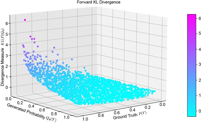
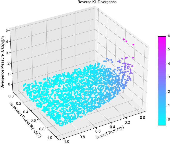
Here is a fact that surprises most students the first time they see it: \(D_{KL}(P\|Q)\) and \(D_{KL}(Q\|P)\) are, in general, two different numbers. KL divergence measures a kind of "distance" between distributions, but it is not a true distance metric — it is not symmetric. Swapping which distribution you call \(P\) and which you call \(Q\) changes the answer. This is not a minor technicality: the two directions penalize mistakes in opposite ways, and that choice quietly shapes what kind of model you end up with. Write both directions out explicitly, side by side, so the difference is visible in the formula itself before we compute anything:
$$\underbrace{D_{KL}(P\|Q)=\sum_x P(x)\log\frac{P(x)}{Q(x)}}_{\text{"Forward" KL — weighted by }P(x)} \qquad\qquad \underbrace{D_{KL}(Q\|P)=\sum_x Q(x)\log\frac{Q(x)}{P(x)}}_{\text{"Reverse" KL — weighted by }Q(x)}$$Both sums run over the exact same log-ratio-flavored quantity, but each one is weighted by a different distribution — the first by \(P\), the second by \(Q\). Since a term weighted by a near-zero number contributes almost nothing to the sum no matter how large the rest of that term is, which distribution does the weighting turns out to control everything.
6.1 First, prove to yourself the two numbers really differ
Before any conceptual discussion, let's just compute both directions for one concrete pair of distributions and see that they are not equal. Suppose the true label distribution over {bike, not-bike} is \(P=[0.9,\,0.1]\) (genuinely 90% likely to be a bike), and the model's current prediction is the under-confident \(Q=[0.6,\,0.4]\).
Forward KL, \(D_{KL}(P\|Q)\) — weighted by \(P\):
$$0.9\log\frac{0.9}{0.6} + 0.1\log\frac{0.1}{0.4} = 0.9(0.4055) + 0.1(-1.3863) = 0.3649 - 0.1386 = \mathbf{0.2263}$$
Reverse KL, \(D_{KL}(Q\|P)\) — same two outcomes, weighted by \(Q\) instead:
$$0.6\log\frac{0.6}{0.9} + 0.4\log\frac{0.4}{0.1} = 0.6(-0.4055) + 0.4(1.3863) = -0.2433 + 0.5545 = \mathbf{0.3112}$$
Same two distributions, same two outcomes — but \(0.2263 \ne 0.3112\). The two directions are not interchangeable. Notice why they differ: the "not-bike" outcome (where the mismatch is largest, 0.1 vs 0.4) gets weight 0.1 in the forward sum but weight 0.4 in the reverse sum — reverse KL lets that badly-mismatched outcome contribute nearly 4× more to the total, simply because \(Q\) itself assigns more probability there.
Recall Section 5: minimizing cross-entropy is exactly minimizing \(D_{KL}(P\|Q)\) — the forward direction, weighted by the true distribution \(P\). That's not an arbitrary convention. In supervised learning, \(P\) (the true label distribution) is fixed and known from the data, while \(Q\) (the model's prediction) is what we're adjusting — so weighting the loss by the fixed, known \(P\) is the only direction that makes sense when \(P\) is data, not a second model we're also trying to fit. The reverse direction becomes relevant in settings where both distributions are model outputs (generative modeling, Section 6.2 below).
6.2 The bigger picture: mean-seeking vs. mode-seeking
The asymmetry above has a striking visual consequence when the true distribution \(P\) has more than one "peak" (exactly the Gaussian Mixture Model from Section 3). The course slides illustrate this with real data generated from a GMM, fit by logistic regression under each KL direction as the loss. Here is the same experiment, reproduced: let the true distribution \(P\) be a bimodal mixture of two Gaussians (two separate clusters of likely values), and ask what single, unimodal (one-peak) Gaussian \(Q\) each KL direction would prefer.
- Forward KL is "zero-avoiding." In \(D_{KL}(P\|Q)=\sum P(x)\log\frac{P(x)}{Q(x)}\), look at any point \(x\) where the true \(P(x)\) is clearly nonzero (i.e., a real peak) but the candidate \(Q(x)\approx0\). Then \(\log\frac{P(x)}{Q(x)}\to\infty\), and because this term is weighted by the nonzero \(P(x)\), it blows up the whole sum. So minimizing forward KL is terrified of ever assigning near-zero probability to somewhere the true distribution actually has mass — it is forced to spread out and cover every real peak at once, even if that means fitting any single peak poorly. This is exactly the mean-seeking (wide, centered-between-the-modes) curve in the figure above.
- Reverse KL is "zero-forcing." In \(D_{KL}(Q\|P)=\sum Q(x)\log\frac{Q(x)}{P(x)}\), the weighting is by \(Q(x)\) instead. Wherever \(Q(x)\approx0\), that term contributes almost nothing to the sum no matter what \(P(x)\) is there — so reverse KL simply doesn't "notice" or get penalized for a peak of \(P\) that \(Q\) chose to ignore. It is free to collapse onto a single peak and fit that one peak tightly, abandoning the rest. This is exactly the mode-seeking (narrow, locked onto one peak) curve above.
6.3 Made concrete: a "bike or not" classifier, animated
The course slides make this asymmetry concrete with a single running example: a classifier that looks at a photo and decides "is this a bike?" There are two genuinely different ways it can be wrong, and — this is the whole point — forward KL and reverse KL disagree sharply about which one is the emergency.
Two photos, two confident mistakes. For each, we isolate the contribution of the "is it a bike?" outcome to the KL sum — this is the piece of the formula that changes most dramatically between the two mistakes (verified below, computed to 4 decimal places):
- Hallucination — shown the ship, the model confidently insists "that's a bike!": true \(P(\text{bike})=0.02\), model says \(Q(\text{bike})=0.95\).
Forward-KL term \(=P\log(P/Q)=0.02\log(0.02/0.95)=\mathbf{-0.077}\) (tiny — forward KL barely notices).
Reverse-KL term \(=Q\log(Q/P)=0.95\log(0.95/0.02)=\mathbf{+3.668}\) (huge — reverse KL flags this as urgent). - Missed pattern — shown a real bike, the model confidently insists "definitely not a bike": true \(P(\text{bike})=0.98\), model says \(Q(\text{bike})=0.03\).
Forward-KL term \(=0.98\log(0.98/0.03)=\mathbf{+3.417}\) (huge — forward KL flags this as urgent instead).
Reverse-KL term \(=0.03\log(0.03/0.98)=\mathbf{-0.105}\) (tiny — reverse KL barely notices).
The two directions have swapped which mistake they treat as an emergency — exactly the zero-avoiding vs. zero-forcing pattern from Section 6.2, now with a photograph attached to each case. (One honest caveat: these are the individual per-outcome contributions, the cleanest way to see the asymmetry directly. If you sum in the complementary "not-a-bike" outcome too, binary classification's two outcomes are complements of each other, which blurs the total gap somewhat — the dramatic version of this effect is really a many-outcome phenomenon, which is exactly what Section 6.2's continuous figure demonstrates rigorously.)
| Case | Ground truth P(bike) | Model says Q(bike) | Forward-KL term | Reverse-KL term |
|---|---|---|---|---|
| Hallucination — ship called "bike" | → 0 | → 1 | ≈ 0 (calm) | Large (hot) |
| Missed pattern — real bike called "not bike" | → 1 | → 0 | Large (hot) | ≈ 0 (calm) |
| Correct rejection — ship called "not bike" | → 0 | → 0 | ≈ 0 | ≈ 0 |
| Correct detection — bike called "bike" | → 1 | → 1 | ≈ 0 | ≈ 0 |
Standard classifiers train with cross-entropy — forward KL — precisely because we want the model punished hardest for missing real patterns (Section 5's whole point). Some generative-model objectives instead behave like reverse KL, and this is the textbook explanation for a famous failure mode called mode collapse: a generator that only ever produces one safe, plausible kind of output is barely penalized for never generating some of the real diversity in the data — reverse KL only punishes it for producing something implausible, not for narrow-mindedness.
Click through the interactive version below for the reasoning behind each mistake:
7. Binary Cross-Entropy, Closing the Loop
For a binary classification target \(y\in\{0,1\}\) and a model prediction \(Q=P(\hat y=1)\), the true label distribution puts all its probability mass on the single correct value. Plugging this two-outcome case into the general cross-entropy formula \(H(P,Q)=-\sum_x P(x)\log Q(x)\) (summed over the two outcomes, "class 1" with probability \(Q\) and "class 0" with probability \(1-Q\)) gives:
$$L=-\big[y\log Q+(1-y)\log(1-Q)\big]$$
This is exactly the loss function Lecture 8 differentiates step by step to derive backpropagation, and exactly the loss whose gradient with respect to a sigmoid output collapses to the remarkably clean \(\partial L/\partial Z_2 = Q - y\). Everything in this lecture — random variables, distributions, MLE, KL divergence — was building toward this one formula, which is not an arbitrary design choice but the direct consequence of maximizing the likelihood of the true labels under the model.
8. Summary
- A random variable maps outcomes to numbers; discrete ones have a PMF, continuous ones have a PDF (whose height is not a probability — only areas under it are).
- Gaussian Mixture Models represent complex distributions as weighted sums of Gaussians, previewing the general problem of modeling an unknown data distribution.
- Minimizing cross-entropy loss is mathematically equivalent to minimizing KL divergence to the true data distribution, because the true distribution's entropy is a constant with respect to model parameters — this is what makes cross-entropy the natural choice for classification.
- KL divergence is asymmetric: \(D_{KL}(P\|Q)\ne D_{KL}(Q\|P)\) — we confirmed this numerically (0.2263 vs. 0.3112 for the same P, Q).
- Forward KL is zero-avoiding (weighted by \(P\), so it's forced to cover every real mode → mean-seeking, spreads out); reverse KL is zero-forcing (weighted by \(Q\), so it can freely ignore modes \(Q\) doesn't cover → mode-seeking, locks onto one peak).
- Binary cross-entropy, \(L=-[y\log Q+(1-y)\log(1-Q)]\), is the exact loss Lecture 8 backpropagates through.
9. Code: Binary Cross-Entropy and a Manual KL Divergence
The script below computes binary cross-entropy for a small toy prediction, then computes KL divergence by hand on a small discrete distribution and verifies the \(H(P,Q)=H(P)+D_{KL}(P\|Q)\) identity numerically.
import numpy as np

# ---- binary cross-entropy on a toy prediction ----
y = np.array([1, 0, 1, 1])
Q = np.array([0.9, 0.2, 0.6, 0.4])   # model's predicted P(class=1)

bce = -np.mean(y * np.log(Q) + (1 - y) * np.log(1 - Q))
print("Binary cross-entropy loss:", round(bce, 4))

# ---- manual KL divergence on a small discrete distribution ----
# P = true distribution, Q = model distribution, over 4 outcomes
P = np.array([0.10, 0.40, 0.35, 0.15])
Qd = np.array([0.20, 0.30, 0.25, 0.25])
assert np.isclose(P.sum(), 1) and np.isclose(Qd.sum(), 1)

def entropy(p):
    return -np.sum(p * np.log(p))

def cross_entropy(p, q):
    return -np.sum(p * np.log(q))

def kl_divergence(p, q):
    return np.sum(p * np.log(p / q))

H_P   = entropy(P)
H_PQ  = cross_entropy(P, Qd)
D_KL  = kl_divergence(P, Qd)

print(f"\nH(P)          = {H_P:.4f}")
print(f"H(P,Q)        = {H_PQ:.4f}")
print(f"D_KL(P||Q)    = {D_KL:.4f}")
print(f"H(P) + D_KL   = {H_P + D_KL:.4f}  (should equal H(P,Q) above)")
⬇ Download lecture-06-crossentropy-kl.py More resources for this lecture →