LSTM Networks: Gates & Memory
Instead of overwriting the hidden state every timestep, an LSTM cell learns exactly what to forget, what to add, and what to reveal — three learned decisions replacing one blunt overwrite.
Lecture 16 diagnosed the exact mechanism behind the vanishing gradient: a long chain of repeated multiplication by the same weight matrix. LSTM's gates are not a random architectural addition — every one of them exists specifically to replace that repeated multiplication with something closer to addition, so gradients survive the trip backward through time.
- Name and define all four LSTM gates/candidates, and give the intuitive 0/0.5/1 reading of each sigmoid gate.
- Write the cell-state update equation and explain why it is (near-)additive across timesteps.
- Explain precisely why the additive cell-state path fixes the vanishing gradient problem from Lecture 16.
- Compute one full LSTM timestep by hand, gate by gate, with real numbers.
- Cite the original LSTM paper and describe its place in the sequence-modeling toolkit.
1. A Memory Cell With Gates
Lecture 16 showed that a plain RNN's hidden state is rewritten at every timestep by repeated multiplication with the shared weight matrix \(W_h\) — the very thing that causes gradients (and, in practice, long-range memory) to vanish. The Long Short-Term Memory network, introduced by Hochreiter & Schmidhuber, "Long short-term memory," Neural Computation, 9(8):1735–1780, 1997, fixes this with a structural change: alongside the usual hidden state \(h_t\), an LSTM carries a second running signal, the cell state \(C_t\), and uses a small set of learned gates to control, at every timestep, exactly how much of the old memory to keep and how much new information to add.
Picture the sentence "I will swim today" being read one word at a time. At the first timestep ("I"), the cell has almost nothing in memory yet, so it mostly writes new information in. At the second timestep ("will"), it must decide: keep what it has about "I" (the subject), and add information about "will" (future tense) — a running memory is built up incrementally, word by word, gate by gate. That is the intuitive picture; the rest of this lecture makes it precise.
2. The Gates, One at a Time
Every gate below is a small feedforward layer that looks at the same two things — the previous hidden state \(h_{t-1}\) and the current input \(x_t\), concatenated as \([h_{t-1}, x_t]\) — and squashes the result with either a sigmoid (\(\sigma\), output in \((0,1)\)) or a tanh (output in \((-1,1)\)).
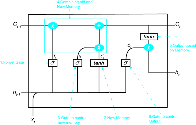
LSTM_CNN.pptx). The six numbered annotations are exactly the six equations below, in the same order: ① forget gate, ② new (candidate) memory, ③ the gate controlling how much new memory to take, ④ combining old and new memory into \(C_t\), ⑤ producing the output from memory, ⑥ the gate controlling how much to output.$$f_t=\sigma\big(W_f[h_{t-1},x_t]+b_f\big)$$
A sigmoid output, applied to the old cell state. Read it directly as a "keep fraction": a value of 0 means forget all previous memory; a value of 1 means keep all previous memory; a value of 0.5 means keep some of the previous memory.
$$\tilde C_t=\tanh\big(W_C[h_{t-1},x_t]+b_C\big)$$
A tanh output — this is proposed new content for the cell state, computed from the current input and previous hidden state. Note it is not yet gated in; that's the next gate's job.
$$i_t=\sigma\big(W_i[h_{t-1},x_t]+b_i\big)$$
Exactly the same 0/0.5/1 reading as the forget gate, but applied to the new candidate memory instead of the old one: 0 = add none of the candidate in; 1 = add all of it; 0.5 = add some of it.
$$C_t=f_t\odot C_{t-1}+i_t\odot\tilde C_t$$
In words: "forget what we don't need from the old memory, and add what we need from the new memory." Both terms are element-wise (\(\odot\)) products of a learned gate with a memory signal, added together — no matrix multiplication of \(C_{t-1}\) happens here at all. This is the structural change that Section 4 will show fixes the vanishing gradient problem.
$$o_t=\sigma\big(W_o[h_{t-1},x_t]+b_o\big)$$
A sigmoid controlling how much of the (tanh-squashed) cell state becomes the visible hidden output: 0 → don't output anything; 1 → output everything; 0.5 → output some.
$$h_t=o_t\odot\tanh(C_t)$$
Every weight matrix above (\(W_f, W_C, W_i, W_o\)) is, like the plain RNN's \(W_h, W_x\), shared across all timesteps. In a real LSTM, \(h_{t-1}, x_t, C_t\) are vectors, and every equation above applies element-wise / via matrix-vector products — for clarity, the worked example in Section 5 treats everything as scalars, but the mechanics generalize directly.
3. All Six Equations, Together
| Gate / signal | Equation | Squashing | Role |
|---|---|---|---|
| Forget | \(f_t=\sigma(W_f[h_{t-1},x_t]+b_f)\) | sigmoid | keep fraction of old \(C_{t-1}\) |
| Candidate | \(\tilde C_t=\tanh(W_C[h_{t-1},x_t]+b_C)\) | tanh | proposed new content |
| Input | \(i_t=\sigma(W_i[h_{t-1},x_t]+b_i)\) | sigmoid | add fraction of candidate |
| Cell state | \(C_t=f_t\odot C_{t-1}+i_t\odot\tilde C_t\) | — | running memory |
| Output | \(o_t=\sigma(W_o[h_{t-1},x_t]+b_o)\) | sigmoid | reveal fraction of \(\tanh(C_t)\) |
| Hidden state | \(h_t=o_t\odot\tanh(C_t)\) | — | visible output |
4. Why This Fixes the Vanishing Gradient Problem
Recall Lecture 16's diagnosis: a plain RNN's gradient backward through time is a product of many Jacobian terms, each involving a repeated multiplication by \(W_h\) — and products of many sub-1 terms vanish geometrically.
Now look at the cell-state update again: \(C_t=f_t\odot C_{t-1}+i_t\odot\tilde C_t\). The path from \(C_{t-1}\) to \(C_t\) is an element-wise multiplication by the forget gate \(f_t\), plus an addition — there is no shared weight matrix repeatedly multiplying the cell state itself at every step. When we backpropagate through the \(C\) path, the gradient at each step is scaled by \(f_t\) (a per-timestep, learned, data-dependent number that can sit close to 1) rather than by the same fixed \(W_h\) every single time.
If the network learns that a particular piece of information should be retained, it can learn to push the relevant forget gate \(f_t\) close to 1 for as many timesteps as needed — letting gradients flow backward through the (near-)additive cell-state path largely unimpeded, instead of being crushed by repeated multiplication with the same weight matrix on every step. The forget gate replaces a fixed, uncontrollable multiplicative shrink with a learned, per-timestep, per-example decision.
5. Worked Numerical Example — One Timestep
Take a single scalar LSTM timestep: previous hidden state \(h_{t-1}=0.2\), previous cell state \(C_{t-1}=0.3\), current input \(x_t=0.5\). Weights (already merging \([h_{t-1},x_t]\) into two scalar coefficients per gate, for arithmetic simplicity):
Forget: \(W_{f,h}=0.5,\ W_{f,x}=0.6,\ b_f=0.1\) |
Input: \(W_{i,h}=0.4,\ W_{i,x}=0.3,\ b_i=0.0\)
Candidate: \(W_{C,h}=0.3,\ W_{C,x}=0.5,\ b_C=0.2\) |
Output: \(W_{o,h}=0.6,\ W_{o,x}=0.4,\ b_o=0.1\)
Now every gate, worked by hand, in order — including the sigmoid/tanh arithmetic itself, not just the final gate value. Recall \(\sigma(z)=\dfrac{1}{1+e^{-z}}\) and \(\tanh(z)=\dfrac{e^{z}-e^{-z}}{e^{z}+e^{-z}}\) (Lecture 5).
First the weighted sum inside the sigmoid:
$$0.5\times0.2 + 0.6\times0.5 + 0.1 = 0.10+0.30+0.10 = \mathbf{0.5}$$
Passed through the sigmoid, this gives \(f_t\approx\mathbf{0.6225}\). If you're already comfortable evaluating \(\sigma(z)=1/(1+e^{-z})\) by hand, skip to the interpretation below; if not, expand for the digit-by-digit arithmetic.
New to this? Expand: σ(0.5) evaluated digit by digit
Now the sigmoid itself, expanded — not just quoted:
$$f_t=\sigma(0.5)=\frac{1}{1+e^{-0.5}}=\frac{1}{1+0.6065}=\frac{1}{1.6065}\approx\mathbf{0.6225}$$
Read as a keep-fraction: the cell keeps about 62% of its old memory \(C_{t-1}\) this step.
Weighted sum:
$$0.4\times0.2 + 0.3\times0.5 + 0.0 = 0.08+0.15+0 = \mathbf{0.23}$$
Passed through the sigmoid, this gives \(i_t\approx\mathbf{0.5573}\). Expand below for the arithmetic if you want it spelled out; otherwise continue to the candidate memory next.
New to this? Expand: σ(0.23) evaluated digit by digit
Sigmoid, expanded:
$$i_t=\sigma(0.23)=\frac{1}{1+e^{-0.23}}=\frac{1}{1+0.7945}=\frac{1}{1.7945}\approx\mathbf{0.5573}$$
About 56% of whatever the candidate memory below turns out to be will be let in.
Weighted sum:
$$0.3\times0.2 + 0.5\times0.5 + 0.2 = 0.06+0.25+0.20 = \mathbf{0.51}$$
Passed through tanh, this gives \(\tilde C_t\approx\mathbf{0.4699}\). If you're already comfortable evaluating \(\tanh(z)=\frac{e^{z}-e^{-z}}{e^{z}+e^{-z}}\) by hand, skip to the interpretation below; if not, expand for the arithmetic.
New to this? Expand: tanh(0.51) evaluated digit by digit
Tanh, expanded using \(e^{0.51}\approx1.6653\) and \(e^{-0.51}\approx0.6005\):
$$\tilde C_t=\tanh(0.51)=\frac{1.6653-0.6005}{1.6653+0.6005}=\frac{1.0648}{2.2658}\approx\mathbf{0.4699}$$
This is the proposed new content — not yet added, since that's the input gate's job (already computed above).
Two products, added — no matrix multiplication of the cell state itself:
$$C_t = \underbrace{0.6225\times0.3}_{\text{kept old memory}} + \underbrace{0.5573\times0.4699}_{\text{added new memory}} = 0.18675 + 0.26192 \approx \mathbf{0.4487}$$
0.18675 came from the 62% of old memory the forget gate kept; 0.26192 came from the 56% of new candidate memory the input gate let in. The new cell state is a learned blend of both, not an overwrite of one by the other.
Weighted sum:
$$0.6\times0.2 + 0.4\times0.5 + 0.1 = 0.12+0.20+0.10 = \mathbf{0.42}$$
Passed through the sigmoid, this gives \(o_t\approx\mathbf{0.6035}\). Expand below for the arithmetic if you want it spelled out; otherwise continue to the final hidden state next.
New to this? Expand: σ(0.42) evaluated digit by digit
Sigmoid, expanded:
$$o_t=\sigma(0.42)=\frac{1}{1+e^{-0.42}}=\frac{1}{1+0.6570}=\frac{1}{1.6570}\approx\mathbf{0.6035}$$
About 60% of the (squashed) cell state will be revealed as the visible hidden state.
First squash the freshly-updated cell state \(C_t=0.4487\) through tanh, giving \(\tanh(C_t)\approx\mathbf{0.4209}\). Expand below for the digit-by-digit arithmetic if you want it; otherwise continue straight to the gating step.
New to this? Expand: tanh(0.4487) evaluated digit by digit
Tanh, expanded using \(e^{0.4487}\approx1.5665\) and \(e^{-0.4487}\approx0.6384\):
$$\tanh(0.4487)=\frac{1.5665-0.6384}{1.5665+0.6384}=\frac{0.9281}{2.2049}\approx\mathbf{0.4209}$$
Then gate it by the output gate:
$$h_t=0.6035\times0.4209\approx\mathbf{0.2540}$$
That single number, \(h_t=0.2540\), is everything this timestep exposes to the next timestep's computations (and, if there's an output layer, to a prediction) — while the richer \(C_t=0.4487\) keeps flowing forward unsquashed as the cell's internal memory.
You can replay the same six gates interactively below — the cell diagram lights up whichever gate is being computed, and the stepper underneath shows the arithmetic behind it:
All six computed values, side by side:
The forget gate \(f_t=0.6225\) keeps a bit more than half of the old cell state; the input gate \(i_t=0.5573\) lets in a bit more than half of the new candidate \(\tilde C_t=0.4699\). The resulting cell state \(C_t=0.4487\) blends both. The output gate \(o_t=0.6035\) then reveals a bit more than half of \(\tanh(C_t)\) as the visible hidden state \(h_t=0.2540\). Every one of these numbers is a genuine, learned decision — not a fixed overwrite.
6. Limitations
- More parameters, more compute. Four weight matrices (\(W_f, W_C, W_i, W_o\)) instead of one — roughly 4× the parameters of a plain RNN cell of the same hidden size.
- Still sequential. Like a plain RNN, \(C_t\) and \(h_t\) cannot be computed before \(C_{t-1}\) and \(h_{t-1}\) exist — no parallelism across the time dimension.
- Mitigates, doesn't eliminate, long-range difficulty. Extremely long sequences (thousands of steps) can still be challenging in practice, which is part of the motivation for attention (Lecture 20).
7. Summary
- An LSTM cell adds a cell state \(C_t\) alongside the hidden state, controlled by three sigmoid gates (forget, input, output) and one tanh candidate.
- Read every sigmoid gate as a 0/0.5/1 "how much" dial: 0 = none, 1 = all, 0.5 = some.
- \(C_t=f_t\odot C_{t-1}+i_t\odot\tilde C_t\) is (near-)additive across timesteps — no repeated matrix multiplication of the cell state — which is exactly why gradients can flow backward through it without vanishing the way they do in a plain RNN.
- Hochreiter & Schmidhuber (1997) introduced this design; it remains the conceptual basis for essentially every gated sequence architecture used since, including the variants in Lecture 18.
8. Code: One LSTM Cell Timestep From Scratch
Reproduces every number in Section 5's worked example exactly.
import numpy as np

def sigmoid(z):
    return 1 / (1 + np.exp(-z))

# ---- state and input (matches the worked example in the lecture) ----
h_prev, C_prev, x = 0.2, 0.3, 0.5

# ---- gate weights (scalar, for a single-unit illustrative LSTM cell) ----
Wfh, Wfx, bf = 0.5, 0.6, 0.1     # forget gate
Wih, Wix, bi = 0.4, 0.3, 0.0     # input gate
WCh, WCx, bC = 0.3, 0.5, 0.2     # candidate memory
Woh, Wox, bo = 0.6, 0.4, 0.1     # output gate

# ---- forward pass through one LSTM timestep, gate by gate ----
f_t = sigmoid(Wfh * h_prev + Wfx * x + bf)
i_t = sigmoid(Wih * h_prev + Wix * x + bi)
C_tilde = np.tanh(WCh * h_prev + WCx * x + bC)
C_t = f_t * C_prev + i_t * C_tilde
o_t = sigmoid(Woh * h_prev + Wox * x + bo)
h_t = o_t * np.tanh(C_t)

print(f"f_t (forget) = {f_t:.4f}")
print(f"i_t (input)  = {i_t:.4f}")
print(f"C~_t (candidate) = {C_tilde:.4f}")
print(f"C_t (cell state)  = {C_t:.4f}")
print(f"o_t (output) = {o_t:.4f}")
print(f"h_t (hidden state) = {h_t:.4f}")

expected = dict(f_t=0.6225, i_t=0.5573, C_tilde=0.4699, C_t=0.4487, o_t=0.6035, h_t=0.2540)
computed = dict(f_t=f_t, i_t=i_t, C_tilde=C_tilde, C_t=C_t, o_t=o_t, h_t=h_t)
for k in expected:
    assert abs(computed[k] - expected[k]) < 1e-3, f"{k} mismatch!"
print("\nAll values match the lecture's hand-worked example.")
⬇ Download lecture-17-lstm-cell.py More resources for this lecture →