Recurrent Neural Networks

Every network so far has treated each input as an isolated snapshot. Sequences — sentences, time series, audio — need a network with memory of what came before.

• Explain why a feedforward network cannot solve tasks where the correct output depends on earlier inputs, not just the current one.
• Write down and interpret the RNN recurrence equations, including which parameters are shared across timesteps.
• "Unroll" a recurrent network through time into an equivalent deep feedforward computation graph.
• Compute a small RNN's hidden states by hand across several timesteps.
• State why weight sharing keeps the parameter count independent of sequence length.
• Name Backpropagation Through Time (BPTT) as the training algorithm and preview the failure mode it exposes (Lecture 16).

1. Why Feedforward Isn't Enough

Every network we have built up to now — Lectures 4 through 14 — is a pure function of its current input. Feed it an image, or a fixed-length feature vector, and it produces an output using only what's in front of it right now. That's exactly right for classifying a single image or a single tabular row. It breaks down the moment order and history matter: time-series forecasting, speech, and — the running example for this module — text.

The instructor's framing is direct: RNNs exist for time-series / sequence analysis — for tasks where "we need to make a prediction based on previous data, not only the current data." A feedforward network has no mechanism to carry information from one input to the next; each forward pass starts from a blank slate.

This is the gap a Recurrent Neural Network (RNN) closes: instead of only mapping input → output, it maintains a running internal state — the hidden state — that is updated at every timestep and carried forward, so past inputs continue to influence future predictions.

2. The Recurrent Equations

An RNN processes a sequence of inputs \(x_1, x_2, \ldots, x_T\) one timestep at a time. At each step it combines the current input with the previous hidden state to produce a new hidden state, then optionally produces an output from that hidden state. Using the instructor's exact notation, with weight matrices \(W_h\) (hidden-to-hidden) and \(W_x\) (input-to-hidden), and an initial hidden state \(h_0\) (usually zero):

$$h_1=\tanh(W_h h_0+W_x x_1) \qquad y_1=W_y h_1$$ $$h_2=\tanh(W_h h_1+W_x x_2) \qquad y_2=W_y h_2$$ $$\ldots \qquad h_t=\tanh(W_h h_{t-1}+W_x x_t) \qquad y_t=W_y h_t$$

The hidden state \(h_t\) is the network's memory: it is a compressed summary of everything the network has seen from \(x_1\) up through \(x_t\). Because \(h_t\) feeds into the computation of \(h_{t+1}\), information from early timesteps can (in principle) still influence outputs many steps later — exactly the capability the "She spoke to her husband" example demanded.

3. Unrolling Through Time

The recurrence \(h_t=\tanh(W_h h_{t-1}+W_x x_t)\) is easiest to reason about — and to train — if we "unroll" it: draw one copy of the computation per timestep, laid out left to right, with the shared weights redrawn at every copy. The result is an equivalent deep feedforward network with \(T\) layers, one layer per timestep, where every layer happens to use identical weights.

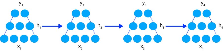
Let's compute this by hand for a simple scalar RNN, so "unrolling" stops being an abstract picture. Take \(W_h=0.5\), \(W_x=0.8\), \(h_0=0\), and a short input sequence \(x_1=1.0,\ x_2=0.5,\ x_3=-0.3,\ x_4=0.2\) (the fourth value is added here purely to extend the pattern one more step). Every timestep applies the exact same rule \(h_t=\tanh(W_h h_{t-1}+W_x x_t)\) — only the two inputs to \(\tanh\) change from step to step, never the weights. Here is the full arithmetic, one timestep at a time:

You can replay the same four steps interactively below — useful for testing yourself before moving on:

4. Why Weight Sharing Is Essential

Imagine instead that each timestep had its own, independently-learned weight matrices: \(W_h^{(1)}, W_h^{(2)}, \ldots\) This design has two fatal problems for sequence data:

• Parameter count would grow with sequence length. A sentence of 5 words and a sentence of 500 words would need entirely different-sized models — impossible, since a language model must handle sentences of any length with one fixed set of parameters.
• Nothing learned at position 3 would transfer to position 30. The whole point of processing "she spoke to her husband" is that the same underlying linguistic rule — "carry subject information forward until it's needed" — should apply no matter where in the sentence it's needed. Tying the weights together forces the network to learn one general-purpose update rule instead of memorizing per-position quirks.

Weight sharing is what lets a single learned function — the RNN cell — be applied uniformly across a sequence of arbitrary length. This is the same intuition behind sharing a convolutional kernel across every spatial location in a CNN (Lecture 13): one small, reusable computation, applied repeatedly.

5. Training: Backpropagation Through Time

How is an RNN trained? Once unrolled, an RNN is a deep feedforward computation graph — so it is trained with exactly the algorithm from Lecture 8: backpropagation. Applied to the unrolled graph, this variant has its own name: Backpropagation Through Time (BPTT).

That accumulation step sounds harmless, but it is where a very specific and important failure mode originates: summing many gradient contributions, each one itself a product of many small terms from the chain rule, over a long sequence. That is precisely the subject of Lecture 16 — The Vanishing/Exploding Gradient Problem, where we'll see exactly why long sequences make this accumulation numerically treacherous.

6. Limitations to Keep in Mind

7. Summary

8. Code: A Scalar RNN Forward Pass

The NumPy script below reproduces the unrolled hand-computation above exactly — run it and confirm \(h_1=0.6640,\ h_2=0.6244,\ h_3=0.0721\) match.

import numpy as np

# Scalar RNN forward pass reproducing the lecture's worked example.
# h_t = tanh(Wh*h_{t-1} + Wx*x_t)   y_t = Wy*h_t
# Wh, Wx, Wy are SHARED across every timestep -- that's the whole point.

Wh, Wx, Wy = 0.5, 0.8, 1.0
h0 = 0.0
xs = [1.0, 0.5, -0.3, 0.2]          # x1..x4

h = h0
hidden_states = []
for t, x in enumerate(xs, start=1):
    h = np.tanh(Wh * h + Wx * x)
    hidden_states.append(h)
    print(f"h{t} = tanh({Wh}*h{t-1} + {Wx}*{x}) = {h:.4f}")

ys = [Wy * h for h in hidden_states]
print("Outputs y1..y4:", [f"{y:.4f}" for y in ys])

# ---- weight sharing: parameter count is independent of sequence length ----
n_params_rnn = 3                     # Wh, Wx, Wy -- fixed, regardless of T
n_params_naive_ff = 3 * len(xs)      # if every timestep had its OWN weights
print(f"RNN params: {n_params_rnn} (shared across all {len(xs)} steps)")
print(f"Naive per-timestep FF params: {n_params_naive_ff} (grows with sequence length)")

⬇ Download lecture-15-rnn-forward.py   More resources for this lecture →