Attention Mechanism & Self-Attention (Transformers)
How a model learns to look back at every word in a sentence and decide, dynamically, which ones matter right now — the single mechanism underneath every modern large language model.
Two unresolved problems are now on the table at once: Lecture 19 showed that Word2Vec gives every word exactly one fixed embedding, no matter the sentence. Lecture 18 showed that an encoder-decoder must compress an entire input sequence into a single fixed-size vector. Attention solves both with one mechanism: let every output look back at the entire input and weigh it dynamically, instead of relying on one static embedding or one compressed summary.
- Explain why Word2Vec's static embeddings (Lecture 19) and the encoder-decoder bottleneck (Lecture 18) both point to the same missing ingredient: attention.
- State the Bahdanau attention formulation — alignment scores, softmax weights, and the context vector — and name the standard family of alignment-score functions.
- Derive scaled dot-product self-attention, \(\text{Attention}(Q,K,V)=\text{softmax}(QK^\top/\sqrt{d_k})V\), and compute it by hand on a real 4-token example.
- Explain why the softmax is scaled by \(\sqrt{d_k}\) and what breaks if you skip it.
- Describe multi-head attention as several independently-learned attention "perspectives" run in parallel, and causal masking as the mechanism that lets decoders train in parallel while respecting left-to-right generation.
- Connect BERT's MLM and NSP pretraining objectives back to cross-entropy (Lecture 6), backprop (Lecture 8), and tokenization (Lecture 19) as one trainable system.
1. From Static to Contextual Embeddings
Lecture 19 gave every word in the vocabulary one fixed embedding, learned by Word2Vec and then frozen. That embedding does not change no matter what sentence the word appears in. Recall the running example: "I went to bank for opening an account" and "I went to bank of a river for the walk" — two completely different senses of "bank," yet Word2Vec hands both occurrences the exact same vector. Separately, Lecture 18 ended on the encoder-decoder bottleneck: a plain sequence-to-sequence model compresses an entire input sequence, however long, into a single fixed-size context vector — and whatever doesn't fit gets lost, especially for long sequences.
Both problems have the same root cause: forcing a single, fixed-size representation to do too much work. And both are solved by the same idea. Instead of handing the decoder one static summary, let the model look back at all positions in the sequence and weigh their relevance dynamically, separately for every step it takes. That dynamic re-weighting is attention. Applied to a sequence's own tokens rather than between an encoder and a decoder, it becomes self-attention — and self-attention is what finally makes word embeddings context-dependent, closing Lecture 19's "bank" problem for good. We build up to that in two stages: first the original, pre-Transformer attention mechanism (Bahdanau attention), then the Transformer's scaled dot-product self-attention, which is the main event of this lecture.
2. Bahdanau Attention: Learning Where to Look
The attention mechanism introduces a set of additional learned parameters whose job is to compute attention weights — numbers that express how important or relevant each element of the input sequence is, at a given decoding step. Instead of the decoder seeing only the encoder's final hidden state (Lecture 18's bottleneck), it now receives a fresh context vector \(c_i\) at every decoding step \(i\), built from the decoder's own previous hidden state and all of the encoder's hidden states — not just the last one.
Let \(T_x\) be the length of the input sequence, \(h_j\) the \(j\)-th encoder hidden state, and \(s_{i-1}\) the decoder's hidden state from the previous step.
$$e_{ij}=\text{align}(s_{i-1}, h_j) \qquad \alpha_{ij}=\frac{\exp(e_{ij})}{\displaystyle\sum_{k=1}^{T_x}\exp(e_{ik})} \qquad c_i=\sum_{j=1}^{T_x}\alpha_{ij}h_j$$\(e_{ij}\) is the alignment score between decoder step \(i\) and encoder position \(j\); softmax turns the row of scores into attention weights \(\alpha_{ij}\) that sum to 1; the context vector \(c_i\) is the resulting weighted sum of encoder states. This should feel familiar — it is exactly the softmax-weighted-sum pattern this lecture will re-derive, in more general form, as self-attention below.
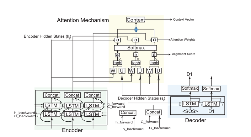
The one open design choice is the alignment function \(\text{align}(\cdot,\cdot)\) itself. Several standard forms exist:
| Name | Form of \(e_{ij}\) | Notes |
|---|---|---|
| Content-base attention | \(\cos(s_{i-1}, h_j)\) | similarity of vectors, no learned parameters |
| Additive (the original Bahdanau form) | \(v_a^\top\tanh(W_a s_{i-1} + U_a h_j)\) | a small learned feed-forward network scores the pair |
| Location-base | \(\text{softmax}(W_a s_{i-1})\) | depends only on the decoder state, not directly on \(h_j\) |
| General | \(s_{i-1}^\top W_a h_j\) | uses a trainable weight matrix \(W_a\) between the two states |
| Dot-product | \(s_{i-1}^\top h_j\) | parameter-free, requires \(s_{i-1}\) and \(h_j\) to have equal dimension |
| Scaled Dot-Product | \(s_{i-1}^\top h_j / \sqrt{n}\) | \(n\) = dimension of the source hidden state — this is exactly what the Transformer generalizes into full self-attention next |
Keep that last row in mind — the rest of this lecture is essentially "scaled dot-product alignment," generalized from a single decoder query against encoder states, to every token in a sequence querying every other token, all at once, with the query/key/value roles themselves learned. That generalization is the Transformer.
3. The Transformer Architecture
The Transformer was introduced by Vaswani et al. in "Attention Is All You Need."† It replaces recurrence entirely — no RNN, no LSTM cell, nothing processes the sequence step by step. Instead, every token attends directly to every other token in a single operation, which is both more expressive and vastly more parallelizable than Lecture 15–18's recurrent architectures.
The architecture has two modules, encoder and decoder, each a stack of 6 identical layers. Each encoder layer has exactly two sub-layers: a self-attention mechanism and a feed-forward network. A residual ("skip") connection wraps each sub-layer, followed by layer normalization:
$$\text{LayerNorm}\big(x+\text{Sublayer}(x)\big)$$The decoder repeats this pattern but inserts a third sub-layer between the two: multi-head attention over the encoder's output stack (so the decoder can look back at the source sequence, exactly as Bahdanau attention did — just computed the Transformer's way). The decoder's own self-attention sub-layer is additionally masked, a detail we return to in Section 6.
| Block | Sub-layers (in order) | Sees future tokens? |
|---|---|---|
| Encoder layer (×6) | Self-attention → Feed-forward | N/A — full sequence given at once |
| Decoder layer (×6) | Masked self-attention → Encoder-decoder attention → Feed-forward | No (masked) |
† The course slides cite this as "Vaswani et al., Attention is all you need" (2023 in the deck's own reference line); the paper was in fact originally published in 2017 (NeurIPS) — the standard, well-known fact — so the 2023 in the source slide most likely reflects when that particular deck was compiled, not the paper's publication date.
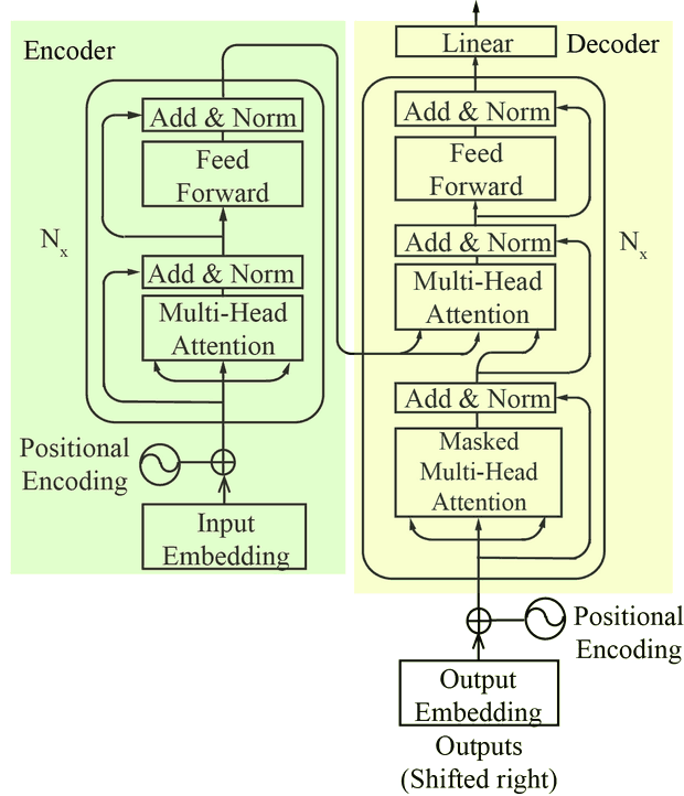
The stack is structurally identical at all 6 levels on each side — same sub-layer types in the same order, same residual+LayerNorm wrapping — but every level has its own independently-learned weights, so stacking lets the token representations get progressively refined, layer after layer. Step through the stack below (the sub-layer sequence shown per card is the encoder's; the decoder repeats the same idea with its extra masked sub-layer):
4. Scaled Dot-Product Self-Attention: A Full Worked Example
Here is the equation that makes the entire Transformer, and by extension every modern large language model, work:
$$\text{Attention}(Q,K,V)=\text{softmax}\!\left(\frac{QK^\top}{\sqrt{d_k}}\right)V$$
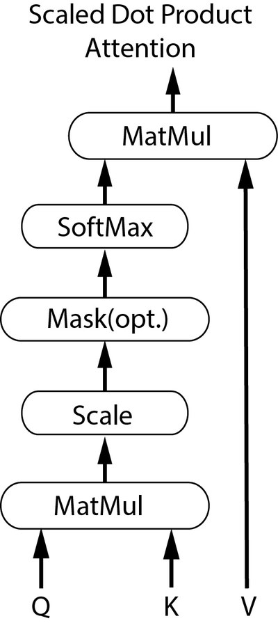
Three matrices — Query \(Q\), Key \(K\), Value \(V\) — combine through a dot product, a scale, a softmax, and a weighted sum, to produce a new set of embeddings in which every token's representation has absorbed information from every other token, weighted by relevance. We now walk through this exactly, step by step, on the course's worked example, sentence "The dog ran fast" — reproducing every number as given on the course slides.
Step 1 — Tokenize & embed
The sentence is first tokenized with a word-piece tokenizer (Lecture 19) into token IDs — the slide's own illustrative snippet shows [1234, 1876, 3456] — which are then looked up in an embedding matrix. The course slide states the embedding dimension used in practice as 768 (this is the real BERT-base embedding size, used here illustratively). For the hand-worked example, a small initial embedding matrix is shown below, truncated to a few dimensions with "…" standing in for the rest of a 768-dimensional row:
Just like Lecture 19's Word2Vec table, this embedding matrix is a set of learned parameters: initialized randomly, then updated by backprop (Lecture 8's algorithm, applied to embedding-table rows) during pre-training. The crucial difference is what happens next. Word2Vec stops here — the vector is frozen per word once training ends. Self-attention is about to take this same fixed input row and blend it with every other token's row, weighted by relevance for this specific sentence — which is what will finally make the output of this layer context-dependent, even though the input embedding you see above is still just one fixed row per token.
Step 2 — Project into Query, Key, and Value matrices
Three separate learned weight matrices \(W_Q, W_K, W_V\) — learned during training, just like \(W_1, W_2\) in Lecture 8's feedforward network — project the same input embedding matrix \(X\) into three different matrices, each a different "view" or projection of the initial embeddings:
$$Q=XW_Q \qquad K=XW_K \qquad V=XW_V$$The course slide's own example numbers (again truncated to a few dimensions, rows in order The / Dog / ran / fast):
Step 3 — Compute attention scores: \(QK^\top\), scale, softmax
First, every query is dotted against every key, giving a raw similarity/score matrix (rows = query token, columns = key token, order The/Dog/ran/fast for both):
These raw scores are then scaled by dividing every entry by \(\sqrt{d_k}\) — the slide explicitly shows this as its own "Scale" step ("÷ \(\sqrt{d_k}\)") before softmax. For the full 768-dimensional case used in practice, \(\sqrt{d_k}=\sqrt{768}\approx 27.7\), so every raw score above would be divided by roughly 27.7 before proceeding — concretely, using the actual raw scores shown in the figure above: the raw score 110 for (The, The) becomes \(110/27.7\approx\mathbf{3.97}\), and the raw score 58 for (The, ran) becomes \(58/27.7\approx\mathbf{2.09}\). Scaling divides every entry in a row by the same constant, so it never changes which score is largest — it only compresses the spread between scores before softmax sees them (more on exactly why that compression matters below).
A dot product between two \(d_k\)-dimensional vectors is a sum of \(d_k\) terms, so its magnitude grows roughly with \(d_k\) (and its variance grows linearly with \(d_k\) under reasonable independence assumptions on the entries). For large \(d_k\) — 768 is large — unscaled dot products can become very large in magnitude. Feeding very large numbers into softmax pushes it into a saturated regime: one entry dominates completely, gradients through the softmax become extremely small, and training stalls. Dividing by \(\sqrt{d_k}\) keeps the variance of the scores roughly constant regardless of embedding dimension, keeping softmax in a well-behaved, trainable regime.
After scaling, a row-wise softmax turns each row of scores into a probability distribution over "which tokens should I attend to." The course slide gives the resulting attention matrix directly:
The intermediate scaling arithmetic on the truncated display values above will not reproduce the exact softmax outputs below — the real computation used the full 768-dimensional \(Q\) and \(K\) vectors, of which we only see a few entries. Use the values below as ground truth, exactly as given on the slide. The important pedagogical content isn't reproducing the last decimal — it's the shape of the result: one row is highly peaked (near-certain self-attention), while others are more spread out across several tokens.
Read it concretely. Row 1, token "The," attends almost entirely to itself — weight 0.99, with the other three tokens receiving essentially nothing (0.0004, 0.0003, 0.0005). That's a common, sensible pattern for a function word with little to disambiguate — "The" doesn't need context from "dog," "ran," or "fast" to know what it means. Row 3, token "ran," spreads its attention much more broadly — 0.38 to itself, 0.269 to "Dog," 0.094 to itself again... (0.38, 0.269, 0.094, 0.25 across The/Dog/ran/fast) — plausibly because a verb's meaning and grammatical role depends heavily on its subject and object elsewhere in the sentence, not just on itself.
Step 3b — The Raw-Score → Scale → Softmax Mechanism, Fully Worked by Hand
Step 3's numbers above are the course slide values, but — as the transparency note already flagged — they come from full 768-dimensional \(Q\) and \(K\) vectors of which the slide (and this page) only shows a few truncated columns, so the exact arithmetic that produces 110 or 0.99 genuinely can't be reproduced from what's on the page. That must not be allowed to hide the mechanism itself. So here is the identical pipeline — dot-product raw score, divide by \(\sqrt{d_k}\), exponentiate, sum, divide — carried out completely, start to finish, on a small, fully-specified toy example with \(d_k=4\) instead of 768, which we construct ourselves precisely so every number is visible. (These toy numbers are illustrative only, not the slide's; only the mechanism should carry over — the same caveat as Step 4's arithmetic below.)
$$Q_{The}=[1.0,\ 0.5,\ -0.5,\ 0.2]$$
$$K_{The}=[0.9,\ 0.4,\ -0.3,\ 0.1] \qquad K_{dog}=[0.2,\ 0.8,\ 0.1,\ -0.4] \qquad K_{ran}=[-0.3,\ 0.2,\ 0.9,\ 0.5] \qquad K_{fast}=[0.4,\ -0.1,\ 0.2,\ 0.7]$$
Multiply matching positions, then add — one dot product per key token:
$$\text{score}(The,The) = (1.0)(0.9)+(0.5)(0.4)+(-0.5)(-0.3)+(0.2)(0.1) = 0.9+0.2+0.15+0.02 = \mathbf{1.27}$$
$$\text{score}(The,dog) = (1.0)(0.2)+(0.5)(0.8)+(-0.5)(0.1)+(0.2)(-0.4) = 0.2+0.4-0.05-0.08 = \mathbf{0.47}$$
$$\text{score}(The,ran) = (1.0)(-0.3)+(0.5)(0.2)+(-0.5)(0.9)+(0.2)(0.5) = -0.3+0.1-0.45+0.1 = \mathbf{-0.55}$$
$$\text{score}(The,fast) = (1.0)(0.4)+(0.5)(-0.1)+(-0.5)(0.2)+(0.2)(0.7) = 0.4-0.05-0.1+0.14 = \mathbf{0.39}$$
So the raw score row for "The" is \([1.27,\ 0.47,\ -0.55,\ 0.39]\) — this is precisely "row \(i\) of \(Q\) dotted with column \(j\) of \(K^\top\) (which is just row \(j\) of \(K\))," the same matrix-multiplication rule from Lecture 4, Section 6, here with \(d_k=4\) instead of 768.
Here \(d_k=4\), so \(\sqrt{d_k}=2\). Divide every entry of the raw score row by 2:
$$[1.27,\ 0.47,\ -0.55,\ 0.39]\ /\ 2 = [\mathbf{0.635},\ \mathbf{0.235},\ \mathbf{-0.275},\ \mathbf{0.195}]$$
Softmax is not a mysterious black box — it is exactly these three arithmetic steps, applied to one row at a time. Step 1, exponentiate each scaled score:
$$e^{0.635}\approx\mathbf{1.887} \qquad e^{0.235}\approx\mathbf{1.265} \qquad e^{-0.275}\approx\mathbf{0.760} \qquad e^{0.195}\approx\mathbf{1.215}$$
Step 2, add up all four exponentiated values to get the row's normalizing constant:
$$\text{sum} = 1.887+1.265+0.760+1.215 = \mathbf{5.127}$$
Step 3, divide each exponentiated value by that sum — this is the entry that actually becomes the attention weight:
$$\alpha_{The,The}=\frac{1.887}{5.127}\approx\mathbf{0.368} \quad \alpha_{The,dog}=\frac{1.265}{5.127}\approx\mathbf{0.247} \quad \alpha_{The,ran}=\frac{0.760}{5.127}\approx\mathbf{0.148} \quad \alpha_{The,fast}=\frac{1.215}{5.127}\approx\mathbf{0.237}$$
Check: \(0.368+0.247+0.148+0.237=1.000\) ✓ — every softmax row must sum to exactly 1 (up to rounding), because turning arbitrary real-valued scores into a valid probability distribution over "which tokens to attend to" is the entire point of the operation. This is the same three-step exponentiate/sum/divide arithmetic that produced the 0.99/0.0004/0.0003/0.0005 row shown in the heatmap above — just computed here on numbers small enough to fully verify by hand.
With toy Value vectors \(V_{The}=[2.0,1.0,0.5,-0.5]\), \(V_{dog}=[0.5,2.0,1.0,0.0]\), \(V_{ran}=[1.0,0.0,2.0,1.5]\), \(V_{fast}=[-1.0,1.5,0.5,2.0]\), dimension 1 of the output for "The" is the weighted sum of dimension-1 values, using exactly the softmax weights just computed:
$$Z_{The,1}=0.368(2.0)+0.247(0.5)+0.148(1.0)+0.237(-1.0)=0.736+0.1235+0.148-0.237\approx\mathbf{0.771}$$
Repeating the same multiply-and-add pattern for the other three dimensions gives \(Z_{The}\approx[0.771,\ 1.217,\ 0.846,\ 0.512]\) — different numbers from the slide's version (different toy inputs), but the identical four-operation mechanism as Step 4's real-slide-number version below.
Step 4 — Weighted sum of Values → new, contextual output embedding
The last step multiplies the attention matrix by the Value matrix: \(Z=\text{Attention}\times V\). Take token "The" (row 1 of the attention matrix: weights 0.99 / 0.0004 / 0.0003 / 0.0005) applied to the four rows of \(V\) shown in Step 2. Showing the arithmetic explicitly for the first dimension (column \(d_1\) of \(V\), values 3.0, 1.4, 5.4, 0.6 for The/Dog/ran/fast):
$$Z_{The,1}=0.99(3.0)+0.0004(1.4)+0.0003(5.4)+0.0005(0.6)=2.97+0.00056+0.00162+0.0003\approx 2.972$$That is close to, but not exactly, the course slide's stated \(Z_{The}\approx[2.96,\ 7.54,\ \ldots,\ 5.45]\) — the small discrepancy comes from the same source we flagged in Step 3: the truncated ellipsis dimensions and display rounding in the slide's numbers, not an error in the method. The mechanism and the near-exact match matter far more than the last decimal.
The output \(Z\) for the word "The" is now a weighted blend of the Value vectors of every word in the sentence, with weights determined by how relevant each word is to "The" in this particular sentence. That is precisely what makes the resulting embedding contextual: the same word "bank" in two different sentences (Lecture 19's example — "I went to bank for opening an account" vs. "I went to bank of a river for the walk") would attend to different surrounding words in each sentence and therefore end up with two different output embeddings — finally solving Word2Vec's static-embedding problem from Section 1.
Walking through exactly why: the projection matrices \(W_Q, W_K, W_V\) are the same learned weights regardless of which sentence "bank" appears in — nothing about them changes between the two sentences. What changes is the Key and Value matrices "bank"'s Query gets dotted against, because those come from \(X W_K\) and \(X W_V\) applied to that sentence's own token embeddings, and the two sentences contain different surrounding tokens. In "I went to bank for opening an account," bank's Query is dotted against Keys for "account," "opening," "for," etc. — words like "account" plausibly produce a high raw score (Step 3's mechanism, exactly as worked out above), so after softmax most of the attention weight lands on "account," and \(Z_{bank}\) ends up as a blend dominated by "account"'s Value vector, i.e. the financial-institution sense. In "I went to bank of a river for the walk," the very same \(W_Q\) produces bank's Query, but it is now dotted against Keys for "river," "walk," etc. instead — "river" plausibly scores highest, so after softmax \(Z_{bank}\) instead ends up dominated by "river"'s Value vector, the geographic sense. Same weights, same equation, same mechanism — but a different sentence supplies a different set of Keys and Values to attend over, which alone is enough to produce two different output vectors for the identical input word.
Made concrete: watch "bank" get two different output vectors
That last paragraph is the whole payoff of this lecture — but it was still only asserted in prose. Here it is made fully numeric, with a small, completely-specified toy example built the same way as Step 3b above (\(d_k=4\), illustrative numbers, not the slide's — same honesty caveat as before). The key experimental control: the Query vector for "bank" is set to the exact same values in both sentences, because it comes from the same input embedding through the same learned \(W_Q\). Only the surrounding words — and therefore their Keys and Values — differ:
$$Q_{bank}=[0.6,\ -0.3,\ 0.8,\ 0.4]\quad\text{— identical in both sentences}$$
Sentence 1 ("...opening an account") supplies context Keys for went, to, opening, account; Sentence 2 ("...bank of a river...") supplies context Keys for went, of, river, walk — note "went" appears in both sentences and, being the same word run through the same \(W_K\), gets the identical Key vector both times. Running the identical score → scale (÷2, since \(\sqrt{d_k}=\sqrt4=2\)) → softmax pipeline from Step 3b independently on each sentence's context (verified by script) gives the attention weights and output vectors below.
"I went to bank for opening an account"
Attention weight peaks on "account" (0.364) — \(Z_{bank}\)'s dimension 1 ends up dominant.
"I went to bank of a river for the walk"
Attention weight peaks on "river" (0.368) — \(Z_{bank}\)'s dimension 3 ends up dominant instead.
Same word, same \(W_Q,W_K,W_V\), same equation — but computing \(Z_{bank}\) for real on the two toy sentences (script-verified, not asserted) gives \(Z_{bank}^{(1)}\approx[1.187,\ 0.272,\ 0.209,\ 0.145]\) for the financial sentence vs. \(Z_{bank}^{(2)}\approx[0.200,\ 0.216,\ 1.070,\ 0.840]\) for the geographic one — Euclidean distance ≈ 1.48, cosine similarity ≈ 0.37 (genuinely different directions, not just a rescaling of the same vector). That is Section 1's promised fix to Word2Vec's static-embedding problem, made numeric rather than only claimed.
5. Multi-Head Attention
One attention computation gives one "view" of how tokens relate to each other. Multi-head attention runs the entire Q/K/V/softmax/weighted-sum process of Section 4 multiple times in parallel, each head with its own independently-learned \(W_Q, W_K, W_V\) projection matrices — so each head is free to specialize in a different kind of relationship: one head might learn to track syntactic subject–verb agreement, another might specialize in coreference (which pronoun refers to which noun), another in something no human-nameable pattern at all. The resulting per-head outputs are concatenated and passed through one more learned linear projection to produce the final multi-head attention output:
$$\text{MultiHead}(Q,K,V)=\text{Concat}(\text{head}_1,\ldots,\text{head}_h)W_O \qquad \text{head}_i=\text{Attention}(QW_Q^i,\,KW_K^i,\,VW_V^i)$$Nothing new is happening arithmetically here — it's exactly Section 4's mechanism, run \(h\) times with different learned weights, then merged. The conceptual leap is what matters: attention is no longer a single fixed lens on the sentence, but several independent, simultaneously-learned lenses whose combined output is far richer than any one of them alone.
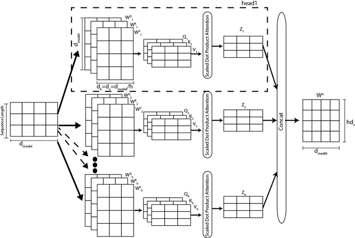
What does "different heads learn different relationships" actually look like on a single sentence? The diagram above shows the plumbing, but not what any individual head's attention pattern looks like — that number isn't on the source slide (it only labels the architecture, not per-head weights), so nothing from it can be reproduced here. What follows instead is illustrative — three constructed, but valid (each row is a genuine softmax distribution, summing to 1.000, verified by script), attention patterns for the same query token "ran" in "The dog ran fast," to make concrete what "several simultaneous lenses" can mean:
6. Masked Multi-Head Attention (Decoder Self-Attention)
In the decoder, self-attention as described above has a problem: at training time the decoder is shown the entire target sequence at once (for efficiency), but it must not be allowed to "see" tokens further to the right that it hasn't generated yet — that would be cheating during training, and is literally impossible at inference time, since those tokens don't exist yet. So the decoder's self-attention sub-layer applies causal masking: right-hand context is hidden during the attention-score computation.
Mechanically, this is simple: before the softmax, a very large negative number (or \(-\infty\)) is added to the raw score of every masked (future) position. After softmax, \(\exp(-\infty)=0\), so those positions' contribution vanishes to (numerically) exactly zero — while every unmasked position's score is untouched and softmax still redistributes correctly among the positions that remain visible. The course slide frames this using <SOS> (start-of-sequence), <PAD>, and <Mask> tokens: at each decoding step only the tokens generated (or known) so far are visible, shown progressively filling in — e.g. 0.99 | *** | *** | *** at the first step, with more real values appearing at each later step as more of the sequence becomes visible, and *** denoting a masked, not-yet-computed position.
Suppose one query position's already-scaled attention scores against four key positions are \([2.0,\ 1.0,\ 3.5,\ 0.5]\), but positions 3 and 4 are future tokens that must be masked. First, add \(-\infty\) to exactly those two entries, leaving the visible entries untouched:
$$[2.0,\ 1.0,\ 3.5,\ 0.5] \ \longrightarrow\ [2.0,\ 1.0,\ -\infty,\ -\infty]$$
Now run the exact same exponentiate → sum → divide softmax mechanism as Step 3b above, on these masked scores. Exponentiating a very large negative number, or \(-\infty\) itself, gives exactly 0:
$$e^{2.0}\approx\mathbf{7.389} \qquad e^{1.0}\approx\mathbf{2.718} \qquad e^{-\infty}=\mathbf{0} \qquad e^{-\infty}=\mathbf{0}$$
$$\text{sum}=7.389+2.718+0+0=\mathbf{10.107}$$
$$\alpha = \left[\frac{7.389}{10.107},\ \frac{2.718}{10.107},\ \frac{0}{10.107},\ \frac{0}{10.107}\right] \approx [\mathbf{0.731},\ \mathbf{0.269},\ \mathbf{0.000},\ \mathbf{0.000}]$$
The masked positions get exactly zero weight — not approximately small, but structurally guaranteed by \(e^{-\infty}=0\) — and the softmax still redistributes the entire probability mass of 1.0, just now only across the two visible positions (0.731 + 0.269 = 1.000). This is the identical arithmetic underlying every 0.99 / 0.55 / 0.45 / … value in the reveal below; only the masked columns' contribution has been forced to zero before the divide step.
The illustrative reveal below shows the same idea on a clean 4-token causal mask (the exact numbers here, beyond the first row's 0.99, are illustrative rather than reproduced from the source table, per the lecture's design — the point is the masking pattern, a lower-triangular reveal):
Because the mask is just an additive matrix applied before one softmax, the entire target sequence's masked self-attention can be computed in a single parallel matrix operation — the mask guarantees position \(i\) mathematically cannot see positions \(>i\), even though all positions are processed simultaneously. This is exactly why decoder-only, autoregressive models (like the GPT family) can be trained efficiently in parallel across an entire sequence, while still respecting the strict left-to-right generation constraint that applies at inference time, one token at a time.
7. BERT: Applying the Encoder Side
BERT (Bidirectional Encoder Representations from Transformers) is built from the encoder portion of the Transformer only — no causal masking is needed, because BERT isn't autoregressively generating text; it's building a representation of a whole sentence it can already see in full. BERT is used to produce context-aware embeddings, directly closing the loop opened in Section 1 / Lecture 19. It is pretrained with two objectives:
| Objective | What happens |
|---|---|
| Masked Language Model (MLM) | The input sentence is tokenized via WordPiece (Lecture 19); 15% of input tokens are masked. BERT's output is an embedding matrix of roughly 512 × 768 (512 = maximum input sequence length, 768 = embedding dimension per token — the same 768 used illustratively in Section 4). The embedding at each masked position is passed to a classifier that predicts the masked word's probability distribution over the full vocabulary — softmax, literally Lecture 6/14's cross-entropy machinery again — loss is computed and weights are updated by backprop (Lecture 8). |
| Next Sentence Prediction (NSP) | The model receives a pair of sentences. In 50% of training pairs the second sentence genuinely follows the first in the original text; in the other 50% it is randomly selected from elsewhere in the corpus. The model is trained to classify which case it is — teaching sentence-level coherence, not just word-level prediction. |
![BERT MLM diagram: the sentence 'after abraham lincoln won the november ...' passes through a Tokenizer producing tokens 0 [CLS], 1 after, 2 abraham, 3 [MASK], up to 511 [PAD]; these feed into BERT, then a Feed-Forward NN, producing a vocab-size output distribution at every position, including at the [MASK] position](assets/img/bert-masked-language-model.jpg)
![BERT NSP diagram: two sentences A and B are joined as [CLS] this is [MASK] to be so [SEP] that [MASK] am done doing [SEP], tokenized and fed through BERT and a Feed-Forward NN + Softmax, producing a 2-way output of 95% Not Next vs 5% Is Next](assets/img/bert-next-sentence-prediction.jpg)
Why this matters pedagogically: BERT is the clearest practical proof that everything covered so far in this course — Lecture 6's cross-entropy, Lecture 8's backprop, Lecture 19's tokenization, and this lecture's self-attention — composes into a single trainable system that produces the contextual word embeddings underlying essentially all modern NLP.
8. Summary & Where This Fits in the Course
Lecture 3 (the perceptron, a single learnable unit) → Lectures 4 & 8 (feedforward networks and backprop — the general trainable-function machinery) → Lecture 6 (cross-entropy, the training objective that drives that machinery) → Lecture 19 (how raw words become vectors in the first place) → Lecture 20, this lecture (how those vectors become context-aware, via attention and self-attention). That progression — a trainable function, a loss to train it against, a way to turn language into numbers, and a mechanism to make those numbers context-sensitive — is the mathematical foundation underneath every modern large language model in production use today.
- Attention replaces a single fixed summary with a dynamic, per-step weighted look-back over the whole sequence — solving both the encoder-decoder bottleneck (Lecture 18) and static word embeddings (Lecture 19).
- Self-attention's core equation, \(\text{Attention}(Q,K,V)=\text{softmax}(QK^\top/\sqrt{d_k})V\), projects the same input into Query/Key/Value views, scores every pair of tokens, scales to keep softmax well-behaved, and produces a weighted blend of Values as the new, contextual output.
- Multi-head attention runs several independently-learned copies of that mechanism in parallel; masked (causal) attention adds \(-\infty\) to future positions' scores so decoders can train in parallel while still respecting left-to-right generation.
- BERT (encoder-only, MLM + NSP) and GPT-style models (decoder-only, causal masking) are the two dominant ways of applying this machinery in practice.
9. Code: Scaled Dot-Product Self-Attention From Scratch
The full Transformer (6-layer encoder/decoder stacks, multi-head attention, positional encodings, layer norm, feed-forward blocks) is too large for a lecture-demo script — see the box below for a complete reference implementation. What follows instead is a small, runnable, self-contained NumPy implementation of the core mechanism this lecture is about: scaled dot-product self-attention, following exactly the four steps of Section 4 (embed → project to Q/K/V → score/scale/softmax → weighted sum of V). It uses made-up, seeded numbers (not the course's truncated 768-dim slide numbers, which can't be reproduced from a small demo) — but the printed attention matrix has the same qualitative shape as the lecture's heatmap: rows that sum to 1, with some peaked and some spread out.
See resources.html for a link to TensorFlow's official "Neural machine translation with a Transformer" Colab tutorial, which implements the complete multi-head, encoder-decoder Transformer end to end.
"""
Lecture 20 - Scaled Dot-Product Self-Attention from scratch (NumPy).

Mirrors the lecture's Section 4 walkthrough:
  Step 1: token embeddings (X)
  Step 2: project to Query, Key, Value   Q = X.Wq   K = X.Wk   V = X.Wv
  Step 3: scores = Q K^T / sqrt(d_k), then row-wise softmax
  Step 4: output Z = Attention @ V  (a context-blended, "contextual" embedding)

The numbers below are made up (seeded random) -- NOT the course's
truncated 768-dim slide numbers, which can't be reproduced exactly from
a small demo. The qualitative shape should match the lecture's heatmap:
rows sum to 1, some rows peaked (near-certain self-attention), some spread
across several tokens.
"""
import numpy as np

np.random.seed(20)


def softmax(x, axis=-1):
    x = x - np.max(x, axis=axis, keepdims=True)   # numerical stability
    e = np.exp(x)
    return e / np.sum(e, axis=axis, keepdims=True)


tokens = ["The", "dog", "ran", "fast"]
n_tokens, d_model, d_k = 4, 8, 8

# ---- Step 1: token embeddings X (n_tokens x d_model) ----
X = np.random.randn(n_tokens, d_model)

# ---- Step 2: learned projection matrices -> Q, K, V ----
Wq = np.random.randn(d_model, d_k) * 0.5
Wk = np.random.randn(d_model, d_k) * 0.5
Wv = np.random.randn(d_model, d_k) * 0.5

Q = X @ Wq
K = X @ Wk
V = X @ Wv

# ---- Step 3: raw scores QK^T, scale by sqrt(d_k), softmax per row ----
scores = Q @ K.T
scaled_scores = scores / np.sqrt(d_k)
attention = softmax(scaled_scores, axis=1)

print("Attention matrix (each row is a probability distribution, sums to 1):")
for tok, row in zip(tokens, attention):
    row_str = "  ".join(f"{v:.3f}" for v in row)
    print(f"  {tok:>5}: {row_str}   sum={row.sum():.3f}")

# ---- Step 4: weighted sum of Values -> contextual output Z ----
Z = attention @ V

print("\nOutput Z (contextual embeddings, one row per token, first 4 dims shown):")
for tok, row in zip(tokens, Z):
    row_str = "  ".join(f"{v:.3f}" for v in row[:4])
    print(f"  {tok:>5}: {row_str} ...")
⬇ Download lecture-20-attention.py More resources for this lecture →