LSTM Variants: BiLSTM, Stacked, Encoder-Decoder, GRU
One LSTM cell, read left-to-right, is only half the picture. Reading both directions, stacking layers, and chaining an encoder into a decoder unlock the architectures behind translation and summarization.
A single LSTM fixes the vanishing-gradient problem, but it still has real blind spots: it only ever sees past context, and an encoder-decoder setup has to compress an entire input sequence into one fixed-size vector. This lecture is a tour of targeted fixes for those two specific remaining weaknesses — and the second one leaves us with a bottleneck problem sharp enough that it demands its own solution (Lecture 20).
- Explain why a standard (unidirectional) LSTM cannot use future context, and why that's sometimes a problem.
- Describe how a Bidirectional LSTM combines two independent LSTMs to see the whole sequence.
- Describe how stacking BiLSTM layers builds progressively more abstract sequence representations.
- Draw and explain the encoder-decoder (seq2seq) architecture, including the role of the <SOS> token and the context vector.
- State the fixed-context bottleneck limitation and connect it to the motivation for attention (Lecture 20).
- Write the GRU equations and describe how it simplifies the LSTM.
1. Past Context Isn't Always Enough
Every LSTM (and plain RNN) we've built so far processes a sequence strictly left to right: at timestep \(t\), the hidden state \(h_t\) can depend on \(x_1,\ldots,x_t\) — the past — but never on \(x_{t+1},\ldots,x_T\) — the future. For generation tasks (predict the next word given only what came before) that's the right constraint. But for many understanding tasks, it's a real handicap.
Consider the word "bank" in isolation. Resolving whether it means a river bank or a financial institution often requires words that appear later in the sentence — "I sat on the bank of the river" vs. "I deposited money at the bank downtown." A purely left-to-right reader only knows "the bank" at the moment it processes that word; the disambiguating evidence hasn't arrived yet.
2. Bidirectional LSTM (BiLSTM)
The fix is architecturally simple: run two independent LSTM cells over the same sequence — one forward (left→right, learning past context, exactly as before) and one backward (right→left, learning future context, processing the sequence in reverse). At every timestep, the two cells' outputs are concatenated to form a representation informed by the entire sequence, not just what came before:
$$h_t^{\text{BiLSTM}} = \big[\,h_t^{\text{forward}}\ ;\ h_t^{\text{backward}}\,\big] \qquad C_t^{\text{BiLSTM}} = \big[\,C_t^{\text{forward}}\ ;\ C_t^{\text{backward}}\,\big]$$Each direction has its own full set of LSTM weights (its own \(W_f,W_C,W_i,W_o\)) — they do not share parameters with each other, only within their own direction across time.
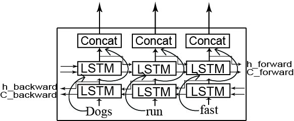
LSTM_CNN.pptx, using the example "Dogs run fast"). Bottom row: the backward LSTM, reading right→left. Middle row: the forward LSTM, reading left→right. Top row: Concat, combining both at every timestep — the same structure animated below for "I / Like / Cats".Walking through the 3-word sequence "I / Like / Cats": the forward LSTM reads left→right, one word ahead of where it started, while the backward LSTM reads the same sentence right→left, independently:
$$h^{\rightarrow}_1=\text{LSTM}_{\text{fwd}}(\text{"I"}) \quad\to\quad h^{\rightarrow}_2=\text{LSTM}_{\text{fwd}}(h^{\rightarrow}_1,\text{"Like"}) \quad\to\quad h^{\rightarrow}_3=\text{LSTM}_{\text{fwd}}(h^{\rightarrow}_2,\text{"Cats"})$$
At \(h^{\rightarrow}_2\) (the word "Like"), only "I" has been seen so far — the future word "Cats" has not entered the computation at all yet.
$$h^{\leftarrow}_3=\text{LSTM}_{\text{bwd}}(\text{"Cats"}) \quad\to\quad h^{\leftarrow}_2=\text{LSTM}_{\text{bwd}}(h^{\leftarrow}_3,\text{"Like"}) \quad\to\quad h^{\leftarrow}_1=\text{LSTM}_{\text{bwd}}(h^{\leftarrow}_2,\text{"I"})$$
At \(h^{\leftarrow}_2\) (also the word "Like", but from the reverse pass), the network has already seen "Cats" — information from later in the sentence that the forward pass at the same position does not have.
Suppose (purely illustrative, not computed from real weights) each direction produces a 3-dimensional hidden vector at the word "Like": \(h^{\rightarrow}_2=[0.62,\,-0.18,\,0.41]\) (built from "I", "Like") and \(h^{\leftarrow}_2=[0.09,\,0.55,\,-0.27]\) (built from "Cats", "Like"). Concatenation simply appends the second vector after the first — no arithmetic combination, just placing both side by side into one longer vector:
$$h_{\text{"Like"}}^{\text{BiLSTM}}=[h^{\rightarrow}_2\,;\,h^{\leftarrow}_2]=[\,0.62,\ -0.18,\ 0.41,\ \ 0.09,\ 0.55,\ -0.27\,]$$
The output dimension doubles (3 + 3 = 6) precisely because nothing is added or averaged — every number computed by both directions is preserved and handed downstream intact. This is why Bidirectional(LSTM(HIDDEN)) in the code below produces a \(2\times\text{HIDDEN}\)-wide output, as the code's comment notes.
You can replay the same steps interactively below — useful for testing yourself before moving on:
At the word "Like", the concatenated state now carries information from both "I" (via the forward direction) and "Cats" (via the backward direction) — exactly the kind of two-sided context needed to resolve ambiguous words like "bank".
3. Stacked BiLSTM
Just as CNNs stack convolutional layers to build progressively more abstract visual features (Lecture 13), BiLSTM layers can be stacked on top of each other: the concatenated forward/backward output of one BiLSTM layer becomes the input sequence fed into the next BiLSTM layer above it. Using the same "I / Like / Cats" example, tokens flow upward through multiple LSTM layers per direction, with a Concat operation combining the forward and backward states at every layer, not just the last one.
Lower layers tend to capture local, syntax-like patterns (e.g. word order, short phrases); higher layers can combine those into more abstract, longer-range semantic patterns — the same "deeper = more abstract" principle that motivates depth in every architecture this course has covered.
4. The Encoder-Decoder (Seq2Seq) Architecture
Stacked BiLSTMs are the building block for one of the most important sequence-to-sequence architectures: the Encoder-Decoder, used for machine translation, summarization, and any task that maps one sequence to another sequence of possibly different length.
- Encoder — a stacked BiLSTM that reads the entire input sequence and compresses it into a single summary: the final concatenated states \(C_{\text{forward}}, C_{\text{backward}}, H_{\text{forward}}, H_{\text{backward}}\).
- Decoder — a unidirectional LSTM chain. It starts from a special <SOS> (start-of-sequence) token, and its initial hidden/cell state is set using the encoder's concatenated context (not zeros). At each step it produces one output token via a softmax layer, then feeds that token back in as the next input — generating the output sequence one token at a time.
This is the classic seq2seq architecture: the encoder's job is understanding, the decoder's job is generation, and the context vector is the single channel connecting the two.
5. The Bottleneck Problem
Notice the architecture's central limitation: no matter how long the input sequence is — five words or five hundred — the entire input must be compressed into one fixed-size context vector before the decoder ever sees it. That vector is an information bottleneck.
In practice, because the encoder's final state is produced by repeatedly overwriting a fixed-size hidden state (Lecture 15/16's recurrence), the words processed last — closest to the end of the sequence — tend to dominate the final context, while information from early words has had many more overwrite-and-forget-gate steps in which to fade. For short sentences this is a minor effect; for long sentences (a paragraph to translate, say) it becomes a serious accuracy problem.
The same reasoning, broken into three steps you can replay interactively:
Instead of forcing the decoder to work from one compressed vector, what if it could look back at all of the encoder's intermediate states, and learn — for each output word it generates — which input words matter most right now? That is precisely the idea Lecture 20 develops: the attention mechanism.
6. GRU — A Simplified Gate (standard textbook material)
The Gated Recurrent Unit (GRU) is not covered in this course's source slides, but it is standard, widely-used material that belongs in any survey of LSTM variants — a simpler gated cell with comparable performance and fewer parameters. It merges the forget and input gates into a single update gate, and merges the cell state and hidden state into one signal:
$$z_t=\sigma(W_z[h_{t-1},x_t]) \qquad r_t=\sigma(W_r[h_{t-1},x_t])$$ $$\tilde h_t=\tanh\big(W[r_t\odot h_{t-1}, x_t]\big) \qquad h_t=(1-z_t)\odot h_{t-1}+z_t\odot\tilde h_t$$Here \(z_t\) (update gate) plays a role similar to the LSTM's forget+input gates combined — it directly interpolates between the old hidden state and the new candidate \(\tilde h_t\) — while \(r_t\) (reset gate) controls how much of the past hidden state is used when computing that candidate. With only two gates and one state (instead of three gates, a candidate, and two states), a GRU has fewer weight matrices to learn, which can mean faster training and less overfitting on smaller datasets, often at little to no cost in accuracy.
| Property | LSTM | GRU |
|---|---|---|
| Gates | 3 (forget, input, output) | 2 (update, reset) |
| Running states | 2 (cell state + hidden state) | 1 (hidden state only) |
| Weight matrices | 4 sets | 3 sets |
| Typical performance | strong | comparable, often similar |
7. Summary
- BiLSTM = two independent LSTMs (forward + backward), concatenated at every timestep — gives access to both past and future context.
- Stacked BiLSTM layers build progressively more abstract sequence representations, the same principle as depth in CNNs.
- Encoder-Decoder: a stacked-BiLSTM encoder compresses the input into a context vector; a unidirectional decoder, seeded from that context and starting at <SOS>, generates output tokens one at a time via softmax.
- The fixed-size context vector is an information bottleneck for long sequences — the direct motivation for attention (Lecture 20).
- GRU: a widely-used simplification merging LSTM's gates and states — fewer parameters, comparable performance.
8. Code: Bidirectional LSTM & a Toy Encoder-Decoder
Illustrative Keras/TensorFlow snippets — architecture wiring, not a full training pipeline.
A complete, trainable seq2seq-with-attention pipeline (data loading, teacher forcing, beam search decoding) is beyond what fits in a single lecture demo. For a full, runnable, Colab-enabled walkthrough, see TensorFlow — Neural Machine Translation with Attention (linked on the resources page).
"""
Lecture 18 -- BiLSTM layer + a toy Encoder-Decoder skeleton (Keras).
Illustrative only: shows how the pieces connect, not a trainable model.
Full trainable seq2seq-with-attention tutorial:
https://www.tensorflow.org/text/tutorials/nmt_with_attention
"""
from tensorflow.keras import layers, Model

VOCAB_SIZE, EMBED_DIM, HIDDEN = 5000, 64, 128

# ---- 1. A Bidirectional LSTM layer (Section 2) ----
inputs = layers.Input(shape=(None,), dtype="int32")
x = layers.Embedding(VOCAB_SIZE, EMBED_DIM, mask_zero=True)(inputs)
bilstm_out = layers.Bidirectional(layers.LSTM(HIDDEN, return_sequences=True))(x)
# bilstm_out shape: (batch, time, 2*HIDDEN) -- forward/backward concatenated
bilstm_model = Model(inputs, bilstm_out, name="bilstm_demo")
bilstm_model.summary()

# ---- 2. A minimal Encoder-Decoder skeleton (Section 4) ----
# Encoder: (Bi)LSTM compresses the source sequence into final states.
enc_inputs = layers.Input(shape=(None,), name="encoder_tokens")
enc_emb = layers.Embedding(VOCAB_SIZE, EMBED_DIM, mask_zero=True)(enc_inputs)
enc_out, fh, fc, bh, bc = layers.Bidirectional(
    layers.LSTM(HIDDEN, return_state=True))(enc_emb)
state_h = layers.Concatenate()([fh, bh])   # H_forward || H_backward
state_c = layers.Concatenate()([fc, bc])   # C_forward || C_backward

# Decoder: unidirectional LSTM, initialised from the encoder's context,
# starts from a  token (handled upstream in the input pipeline),
# predicts one token at a time via softmax.
dec_inputs = layers.Input(shape=(None,), name="decoder_tokens")  # teacher-forced
dec_emb = layers.Embedding(VOCAB_SIZE, EMBED_DIM, mask_zero=True)(dec_inputs)
dec_lstm = layers.LSTM(2 * HIDDEN, return_sequences=True)
dec_out = dec_lstm(dec_emb, initial_state=[state_h, state_c])
dec_softmax = layers.Dense(VOCAB_SIZE, activation="softmax")(dec_out)

seq2seq = Model([enc_inputs, dec_inputs], dec_softmax, name="encoder_decoder_demo")
seq2seq.summary()
⬇ Download lecture-18-bilstm-seq2seq.py More resources for this lecture →