Boltzmann Machines, Energy-Based Models, Contrastive Divergence & Deep Belief Networks
Borrowing a page from physics: define an energy over configurations, let low-energy states be probable, and learn by nudging the energy landscape with real data.
Lecture 21 found structure in unlabeled data through competition and geometric proximity — the nearest prototype wins. This lecture approaches the same "no labels" problem from a completely different direction, borrowed from physics: instead of geometric distance, model the data with a notion of energy and probability, so the network doesn't just organize data — it can learn to generate it.
- Explain the Boltzmann distribution and how energy-based models turn "low energy ⇒ high probability" into a training principle.
- Write the full Boltzmann Machine energy function and identify why full connectivity makes exact training intractable.
- Derive the Restricted Boltzmann Machine's simplified energy function and its tractable conditional-independence property.
- Derive, step by step, the positive-phase / negative-phase gradient of the RBM log-likelihood.
- Compute one full Contrastive Divergence (CD-1) update by hand on a 2-visible / 1-hidden RBM.
- Describe how Deep Belief Networks stack RBMs via greedy layer-wise pretraining, and why this mattered historically.
1. Energy-Based Models & the Boltzmann Distribution
Every model in this course so far has been trained by directly minimizing a loss between a prediction and a target. Energy-based models take a different route, borrowed from statistical mechanics: physical systems tend to settle into low-energy states — a ball rolls downhill, a magnet aligns its spins to minimize energy. The Boltzmann distribution formalizes this: the probability of a system being found in a particular state is
$$P(\text{state})=\frac{e^{-E(\text{state})/kT}}{Z}$$where \(E\) is the energy of that state, \(k\) is the Boltzmann constant, \(T\) is temperature, and \(Z=\sum_{\text{all states}}e^{-E(\text{state})/kT}\) is the partition function — the normalizing constant that sums \(e^{-E/kT}\) over every possible state so probabilities sum to 1. The interpretation is direct: lower energy makes \(e^{-E}\) larger, which makes that state more probable.
In deep learning we drop the physical constants — \(k\) and \(T\) are simply absorbed into how the energy function is scaled — and write the relationship in its cleanest form:
$$P(\text{state})\propto e^{-E(\text{state})}$$Everything so far has been the formula. Here is what it actually does: a toy system with 5 possible configurations (states A–E), each with its own assigned energy. Press play and watch the system wander through configurations and settle where the formula says it must — the lowest-energy valley:
Boltzmann Machines take their name, and this core principle, directly from this distribution: they define a learnable energy function over configurations of binary units, and training shapes that energy landscape so that configurations resembling real data end up with low energy (hence high probability).
2. The Boltzmann Machine: Architecture & Energy Function
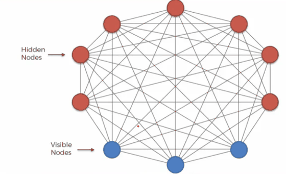
A Boltzmann Machine has two layers of binary stochastic units:
- Visible units \(v_i\in\{0,1\}\) — represent observed data: pixels, features, ratings.
- Hidden units \(h_j\in\{0,1\}\) — learn latent structure that explains dependencies among the visible units, adding stochasticity so the model can represent complex distributions.
Connections are symmetric (\(w_{ij}=w_{ji}\)) and there are no self-connections. The full energy function includes every possible pairwise interaction: visible biases, hidden biases, visible–visible interactions, hidden–hidden interactions, and visible–hidden interactions:
and the probability of a joint configuration follows the Boltzmann form directly:
$$P(v,h)=\frac{e^{-E(v,h)}}{Z}$$What do the visible units actually represent? It depends on the data:
| Data type | Visible unit \(v_i\) semantics |
|---|---|
| Binary images (e.g. MNIST) | \(v_i\) = pixel on/off |
| Text / bag-of-words | \(v_i\) = word present/absent |
| Recommendation systems | \(v_i\) = binarized user–item rating |
| Sensor / speech data | continuous — needs a Gaussian RBM variant |
3. Why Binary Units? & RBM Variants for Other Data
Binary units were the historical default (Hinton & Sejnowski, 1983) for several concrete reasons: they keep the pairwise energy terms simple; they admit an easy, well-defined stochastic sampling rule via the sigmoid, \(P(v_i=1\mid h)=\sigma\!\big(a_i+\sum_jw_{ij}h_j\big)\); they're cleanly compatible with the Boltzmann distribution's exponential form; and they carry a loose biological analogy to a neuron that either fires or doesn't.
Real data isn't always binary, so the RBM family (introduced formally in Section 5) has variants for other data types:
| Variant | Data type | Mechanism |
|---|---|---|
| Bernoulli RBM | Binary | Sigmoid units (the default form) |
| Gaussian–Bernoulli RBM | Continuous | e.g. raw pixel intensities |
| Softmax / Multinomial RBM | Categorical, one-hot | e.g. words / topics |
| ReLU / Rectified RBM | Non-negative continuous | Sparse coding |
4. Applications
Boltzmann Machines and RBMs have been used for: feature / representation learning (unsupervised pretraining of features later used by another model), data generation (sampling new visible patterns from the learned distribution), collaborative filtering (RBMs were famously used in the Netflix Prize recommendation system), anomaly detection (high-energy states correspond to unlikely, i.e. anomalous, inputs), and speech, text, and biological sequence modeling.
5. From Boltzmann Machines to RBMs
The full Boltzmann Machine, as elegant as its energy function is, does not scale. Full connectivity means every unit depends on every other unit, which creates exponentially many possible joint states; computing the partition function \(Z\) — a sum over all of them — becomes intractable for anything beyond a toy size. Training requires long Markov-chain (Gibbs sampling) runs just to approximate the expectations the gradient needs, which is slow and doesn't scale past a few dozen units, precisely because visible–visible and hidden–hidden connections make every unit mutually dependent on every other.
The Restricted Boltzmann Machine (RBM) removes all intra-layer connections — no visible–visible links, no hidden–hidden links — keeping only visible–hidden connections. The result is a bipartite graph, and a much simpler energy function:
This restriction has one crucial payoff: given \(v\), all the hidden units become conditionally independent of each other (and symmetrically, given \(h\), all visible units become conditionally independent of each other). That's what makes RBM training tractable — the entire hidden layer can be sampled in a single parallel step given the visible layer, and vice versa, with no need to sample one unit at a time while holding the rest fixed.
6. Learning Objective & Gradient Derivation
We want to maximize the log-likelihood of the data under the model, \(\log P(v)\), where \(P(v)=\frac1Z\sum_he^{-E(v,h)}\). It's convenient to write this using the free energy \(F(v)=-\log\sum_he^{-E(v,h)}\), so that \(\log P(v)=-F(v)-\log Z\). Since this splits into two separate terms, we differentiate each one with respect to a weight \(w_{ij}\) in turn: \(\frac{\partial\log P(v)}{\partial w_{ij}}=-\frac{\partial F(v)}{\partial w_{ij}}-\frac{\partial\log Z}{\partial w_{ij}}\). Every algebraic step of both halves is worked out below.
By definition \(F(v)=-\log\sum_he^{-E(v,h)}\). Differentiating a \(-\log(\cdot)\) of a sum brings down a \(1/(\cdot)\) times the derivative of the sum, and the derivative of each \(e^{-E(v,h)}\) term with respect to \(w_{ij}\) is \(e^{-E(v,h)}\cdot(-\partial E(v,h)/\partial w_{ij})\) by the chain rule. The two minus signs cancel, and \(e^{-E(v,h)}/\sum_{h'}e^{-E(v,h')}\) is exactly the definition of \(P(h\mid v)\):
$$\frac{\partial F(v)}{\partial w_{ij}}=\sum_h P(h\mid v)\,\frac{\partial E(v,h)}{\partial w_{ij}}$$
For an RBM, the only term of \(E(v,h)=-\sum_ia_iv_i-\sum_jb_jh_j-\sum_{i,j}v_iw_{ij}h_j\) that depends on \(w_{ij}\) is \(-v_iw_{ij}h_j\), whose derivative is simply \(-v_ih_j\). Substituting into Step 1 and flipping the sign on both sides:
$$-\frac{\partial F(v)}{\partial w_{ij}}=\sum_h P(h\mid v)\,v_ih_j=\mathbb{E}_{h\mid v}[v_ih_j]$$
In this expectation, \(v\) is clamped to a specific data point (we're differentiating \(\log P(v)\) for a fixed \(v\)), so \(v_i\) is a plain number, not a random variable — it factors straight out of the sum over \(h\). What remains, \(\sum_hP(h\mid v)h_j\), is just the expected value of the binary variable \(h_j\), which for a 0/1 variable is exactly its probability of being 1:
$$\mathbb{E}_{h\mid v}[v_ih_j]=v_i\cdot\mathbb{E}_{h\mid v}[h_j]=v_i\cdot P(h_j{=}1\mid v)$$
Because an RBM has no hidden–hidden connections (Section 5), \(P(h_j{=}1\mid v)\) depends only on \(v\) and neuron \(j\)'s own bias/weights — it collapses to a single sigmoid, with no other hidden units involved:
$$P(h_j{=}1\mid v)=\sigma\!\Big(b_j+\sum_i w_{ij}v_i\Big)$$
This is exactly the tractable, single-step-sampleable conditional made possible by removing intra-layer connections. Combining Steps 3–4, \(-\partial F(v)/\partial w_{ij}=v_i\cdot P(h_j{=}1\mid v)\) is now something we can compute exactly, in one pass, for any clamped data point \(v\) — this is the positive phase.
Now the second half. \(Z=\sum_{v,h}e^{-E(v,h)}\) sums over every possible joint configuration, not just those consistent with one data point. Differentiating \(\log Z\) follows the identical chain-rule pattern as Step 1 — but this time the sum ranges over all \((v,h)\) pairs, and \(e^{-E(v,h)}/Z\) is exactly the model's own joint distribution \(P_{\text{model}}(v,h)\). Substituting the same energy derivative from Step 2 (\(-v_ih_j\)) and flipping signs the same way:
$$\frac{\partial \log Z}{\partial w_{ij}}=\sum_{v,h} P_{\text{model}}(v,h)\,v_ih_j=\langle v_ih_j\rangle_{\text{model}}$$
This is an expectation over the model's own distribution, not the data — computing it exactly requires summing over every possible \((v,h)\), which is intractable for anything beyond a toy-sized RBM. This is the negative phase, and it is the entire reason Contrastive Divergence (Section 7) exists.
Recall \(\frac{\partial\log P(v)}{\partial w_{ij}}=-\frac{\partial F(v)}{\partial w_{ij}}-\frac{\partial\log Z}{\partial w_{ij}}\). Substituting the results of Step 4 (\(-\partial F/\partial w_{ij}=v_i\cdot P(h_j{=}1\mid v)=\langle v_ih_j\rangle_{\text{data}}\)) and Step 5 gives the full gradient:
$$\frac{\partial\log P(v)}{\partial w_{ij}}=\underbrace{\langle v_ih_j\rangle_{\text{data}}}_{\text{Positive Phase}}-\underbrace{\langle v_ih_j\rangle_{\text{model}}}_{\text{Negative Phase}}$$ Increase \(w_{ij}\) if \(v_i\) and \(h_j\) co-occur more in the real data than the model currently predicts; decrease it if the model over-predicts that co-occurrence.
You can replay the same five steps interactively below — useful for testing yourself before moving on:
The positive phase is easy: clamp the visible units to a real data point and compute the exact hidden-unit probabilities — a single, exact computation. The negative phase is the problem: it is an expectation over the model's own distribution, which would require running a long Gibbs-sampling chain to equilibrium to get an unbiased sample — computationally expensive, and the core bottleneck in training any Boltzmann-family model.
7. Contrastive Divergence (CD-k)
Contrastive Divergence is the practical fix that made RBMs trainable at scale: instead of running Gibbs sampling all the way to equilibrium for the negative phase, run just \(k\) steps — most commonly \(k=1\), "CD-1" — starting from the real data point (not from random noise), and treat that short chain's endpoint as a cheap stand-in for the negative-phase expectation.
- Start at the data point \(v^{(0)}\), sample \(h^{(0)}\sim P(h\mid v^{(0)})\).
- Run \(k\) Gibbs steps: \(v^{(t+1)}\sim P(v\mid h^{(t)})\), then \(h^{(t+1)}\sim P(h\mid v^{(t+1)})\), for \(t=0,\dots,k-1\).
- Approximate the negative phase: \(\langle v_ih_j\rangle_{\text{model}}\approx v_i^{(k)}\cdot P(h_j=1\mid v^{(k)})\).
This gives a simple, fully computable update rule:
$$\Delta w_{ij}=\eta\Big[v_i^{(0)}P(h_j{=}1\mid v^{(0)})-v_i^{(k)}P(h_j{=}1\mid v^{(k)})\Big]$$CD-k, in one sentence: deepen valleys at real data (positive phase) and shrink hills at model samples (negative phase).
8. Worked Example: One Full CD-1 Step
A tiny RBM: 2 visible units (\(v_1,v_2\)), 1 hidden unit (\(h\)). Weights \(W=[0.8,\ 0.4]\) (\(w_1\) connects \(v_1\)–\(h\), \(w_2\) connects \(v_2\)–\(h\)), biases \(a_1=a_2=b=0\), learning rate \(\eta=0.1\). Data (clamped): \(v^{(0)}=(1,0)\). Every sigmoid below is computed the same way: evaluate the exponent, exponentiate, add 1, divide into 1 — spelled out in full so nothing is hidden.
Weighted input to \(h\): \(b+w_1v_1+w_2v_2 = 0+0.8(1)+0.4(0)=0.8\). Now the sigmoid, in full:
$$\hat h^{(0)}=P(h{=}1\mid v^{(0)})=\sigma(0.8)=\frac{1}{1+e^{-0.8}}=\frac{1}{1+0.4493}=\frac{1}{1.4493}\approx\mathbf{0.689974}$$
The positive-phase associations \(\langle v_ih\rangle_{\text{data}}=v_i^{(0)}\cdot\hat h^{(0)}\), one per visible unit:
$$\langle v_1h\rangle_{\text{data}}=1\times0.689974=\mathbf{0.689974}\qquad\qquad \langle v_2h\rangle_{\text{data}}=0\times0.689974=\mathbf{0.000000}$$
With no visible–visible connections, each visible unit's reconstruction probability depends only on \(\hat h^{(0)}\) and its own weight — \(P(v_i{=}1\mid h)=\sigma(a_i+w_i\hat h^{(0)})\):
$$\tilde v_1=\sigma(0.8\times0.689974)=\sigma(0.551979)=\frac{1}{1+e^{-0.551979}}=\frac{1}{1+0.5758}=\frac{1}{1.5758}\approx\mathbf{0.634595}$$
$$\tilde v_2=\sigma(0.4\times0.689974)=\sigma(0.275990)=\frac{1}{1+e^{-0.275990}}=\frac{1}{1+0.7588}=\frac{1}{1.7588}\approx\mathbf{0.568563}$$
Then resample the hidden unit from this reconstruction — weighted input \(=0.8(0.634595)+0.4(0.568563)=0.507676+0.227425=0.735101\):
$$\hat h^{(1)}=\sigma(0.735101)=\frac{1}{1+e^{-0.735101}}=\frac{1}{1+0.4795}=\frac{1}{1.4795}\approx\mathbf{0.675924}$$
CD-1 uses the reconstruction \(\tilde v\) and resampled \(\hat h^{(1)}\) in place of a true equilibrium sample:
$$\langle v_1h\rangle_{\text{model}}\approx0.634595\times0.675924\approx\mathbf{0.428938}\qquad\qquad \langle v_2h\rangle_{\text{model}}\approx0.568563\times0.675924\approx\mathbf{0.384305}$$
$$\Delta W_1=0.1(0.689974-0.428938)=0.1(0.261036)\approx\mathbf{+0.026104}$$
$$\Delta W_2=0.1(0.000000-0.384305)=0.1(-0.384305)\approx\mathbf{-0.038431}$$
$$\Delta a_1=0.1(1-0.634595)=0.1(0.365405)\approx\mathbf{+0.036541}$$
$$\Delta a_2=0.1(0-0.568563)=0.1(-0.568563)\approx\mathbf{-0.056856}$$
$$\Delta b=0.1(0.689974-0.675924)=0.1(0.014050)\approx\mathbf{+0.001405}$$
You can replay the same four stages interactively below — useful for testing yourself before moving on, and it drives the diagram above:
\(W_1\) strengthens (Δ = +0.0261): the data co-activates \(v_1\) and \(h\) more strongly than the model's own reconstruction does. \(W_2\) weakens (Δ = −0.0384): the model over-predicts \(v_2\) activating \(h\), relative to the data, so training pulls that connection down.
9. Deep Belief Networks (DBN)
DBNs are not covered in the local course slides. What follows is standard textbook material, kept deliberately brief relative to the RBM/CD content above.
A Deep Belief Network is simply a stack of RBMs, trained greedily, one layer at a time: train the first RBM directly on the raw data; then freeze it, run the data through it to get hidden-layer activations, and treat those activations as the "data" for training a second RBM stacked on top; repeat for as many layers as desired. Once every layer has been pretrained this way, the whole stack can be "unrolled" into a single deep network and fine-tuned end-to-end with ordinary backpropagation — typically with a supervised classifier layer added on top for the final task.
Historically (Hinton, Osindero & Teh, 2006), this greedy layer-wise pretraining was one of the first techniques that made training genuinely deep networks practical at all — before that, deep networks were notoriously hard to train from a random initialization. Better weight-initialization schemes, ReLU activations, batch normalization, and residual connections (all covered earlier in this course) have since made layer-wise RBM pretraining largely unnecessary for most modern architectures — but it remains a historically important idea, and the direct ancestor of the encoder-style unsupervised pretraining still used in some settings today.
Summary
- Energy-based models define \(P(\text{state})\propto e^{-E(\text{state})}\) — training shapes the energy landscape so real data sits in low-energy valleys.
- Full Boltzmann Machines are intractable because of visible–visible and hidden–hidden connections; RBMs restrict connectivity to bipartite visible–hidden links, making sampling one layer at a time exact and parallel.
- The RBM gradient splits into a tractable positive phase (data-clamped) and an intractable negative phase (requires sampling the full model) — Contrastive Divergence approximates the negative phase with just \(k\) Gibbs steps starting from the data.
- DBNs stack RBMs via greedy layer-wise pretraining, then fine-tune with backprop — historically pivotal for training deep nets, though largely superseded by modern initialization and normalization techniques.
10. Code: One CD-1 Step From Scratch
The NumPy code below reproduces every number in the Section 8 worked example exactly — run it and confirm the printed values against the hand derivation.
import numpy as np

def sigmoid(z): return 1 / (1 + np.exp(-z))

# ---- tiny RBM: 2 visible units, 1 hidden unit ----
W = np.array([0.8, 0.4])   # w1 (v1-h), w2 (v2-h)
a = np.array([0.0, 0.0])   # visible biases
b = 0.0                    # hidden bias
eta = 0.1
v0 = np.array([1.0, 0.0])  # clamped data point

# ---- positive phase ----
h0_prob = sigmoid(b + W @ v0)
pos_assoc = v0 * h0_prob
print("h0 =", h0_prob, " positive  =", pos_assoc)

# ---- negative phase: one Gibbs step (CD-1) ----
v1_prob = sigmoid(a + W * h0_prob)          # reconstruct visible units
h1_prob = sigmoid(b + W @ v1_prob)          # resample hidden from reconstruction
neg_assoc = v1_prob * h1_prob
print("v_tilde =", v1_prob, " h1 =", h1_prob, " negative  =", neg_assoc)

# ---- CD-1 parameter updates ----
dW = eta * (pos_assoc - neg_assoc)
da = eta * (v0 - v1_prob)
db = eta * (h0_prob - h1_prob)
print("dW =", dW, " da =", da, " db =", db)

W_new = W + dW
print("Updated W =", W_new)
⬇ Download lecture-22-cd1-rbm.py More resources for this lecture →