CNNs: Motivation & Architecture
Why feeding raw pixels into a dense network is a losing proposition — and the four-layer blueprint, inspired by the visual cortex, that made computer vision tractable for deep nets.
Lectures 4–11 treated every input as a flat vector of numbers, with no assumption about how those numbers relate to each other. That assumption quietly breaks for images: flattening a photo throws away the fact that nearby pixels are related, and it makes the network gigantic. This lecture is about what changes when the shape of the input actually matters.
- State, with exact numbers, why a dense/feedforward network scales catastrophically on raw image input.
- List the three concrete disadvantages of MLPs for image data, and how convolution fixes each one.
- Trace CNN history from the Neocognitron and biological vision through LeNet-5.
- Describe the generic 4-layer CNN blueprint (Input → Convolution → Pooling → Fully Connected) and the deep pipeline built from it.
- Explain why convolutional layers are parameter-cheap while fully-connected layers dominate parameter count — and how later architectures exploited that.
- Compare AlexNet, VGG16, GoogLeNet and ResNet on accuracy and parameter budget.
1. Why Not Just Use a Dense Network on Images?
Every network we built through Lecture 11 was a stack of fully-connected (dense) layers: flatten the input into a 1D vector, multiply by a weight matrix, repeat. Nothing stops us from doing the same thing to an image — flatten the pixels into one long vector and feed it to an MLP. The reason nobody does this at scale is a matter of simple arithmetic.
Take a modest 224×224 RGB image. Flattened, that is
$$224 \times 224 \times 3 = 150{,}528 \text{ inputs}$$Connect that input vector to a first hidden layer of just 1000 neurons, fully connected, and the weight matrix alone has
$$150{,}528 \times 1000 \approx 150 \text{ million weights}$$— in a single layer, before we've added a second hidden layer, before biases, before the output layer. That's computationally expensive to store and train, and with any realistic (limited) amount of labelled image data, a model with that many free parameters overfits badly.
The parameter count is the headline problem, but it isn't the only one. This breaks down into three concrete disadvantages of MLPs on image data:
- Too many parameters. As above — a fully-connected layer scales as (number of pixels) × (number of hidden units), which explodes for anything but tiny images.
- No notion of local spatial structure. An MLP treats every pixel as an independent input feature; it has no built-in concept of which pixels are neighbors. It cannot exploit the fact that edges, textures and shapes are formed by small groups of nearby pixels. CNNs instead use small filters (e.g. 3×3, 5×5) that look at a local neighborhood at a time, directly encoding "nearby pixels are related."
- No translation invariance. If an MLP learns to recognize a cat when it appears in the top-left of the frame, there is no guarantee it recognizes the same cat shifted to the center of the frame — every pixel position has its own independent weights. A CNN's convolution-plus-pooling combination applies the same filter everywhere in the image and then pools over small neighborhoods, so the same pattern is detected regardless of where it appears.
A dense layer asks "what weight should pixel (117, 203) get?" as if that pixel's meaning were independent of every other pixel. A convolutional layer asks "what small pattern (edge, corner, blob) should I look for, and where in the image does it occur?" — the same question, asked identically at every location. That single change in framing is what makes vision tractable.
2. A Brief History: From Visual Cortex to LeNet-5
CNNs are not a purely mathematical invention — they are directly inspired by biology, and the architecture evolved over three decades before "deep learning" was a common phrase.
- Hubel & Wiesel (1959) studied the cat visual cortex and found two kinds of cells: simple cells that respond to local, orientation-specific edges in a small receptive field, and complex cells that pool the responses of many simple cells to become invariant to the exact position of the edge. This simple-cell → complex-cell hierarchy is the biological blueprint for convolution → pooling.
- Neocognitron (Fukushima, 1980) was the first computational architecture built directly on that biology — layers of "S-cells" (feature detectors, like convolution) alternating with "C-cells" (spatial pooling for invariance), stacked hierarchically.
- Time-Delay Neural Network (Waibel & Hinton, 1987) applied the same idea to sequences: 16 convolution kernels slid over 15-element windows, with the kernel weights shared across every window position and the whole network trained end-to-end with backpropagation. This introduced the crucial engineering idea of learned, shared-weight convolution kernels trained by gradient descent (rather than hand-designed filters).
- First CNN for images (LeCun, 1989) combined convolution, weight sharing and backprop specifically for 2D image recognition (handwritten digits) for the first time.
- LeNet-5 (LeCun, 1989) is the architecture most people mean by "the first CNN" — small, entirely hand-inspectable, and still the cleanest worked example of the pattern. Its own defining choices: 5×5 filters, stride 1, sigmoid nonlinearity, 2×2 stride-2 pooling, grayscale input, and no zero padding (so the feature maps shrink at every convolution).
The classic LeNet-5 layer stack (standard textbook depiction, digit-recognition input) is worth walking through once, because every later CNN is a variation on this same skeleton:
| Layer | Type | Output shape | Filter / pool |
|---|---|---|---|
| Input | Grayscale image | 32×32×1 | — |
| C1 | Convolution | 28×28×6 | 5×5, stride 1 |
| S2 | Pooling | 14×14×6 | 2×2, stride 2 |
| C3 | Convolution | 10×10×16 | 5×5, stride 1 |
| S4 | Pooling | 5×5×16 | 2×2, stride 2 |
| C5 | Convolution (acts as FC) | 120 | 5×5, stride 1 |
| F6 | Fully connected | 84 | — |
| Output | Fully connected | 10 | — |
Notice the pattern that repeats throughout this course: convolution → pooling → convolution → pooling → flatten → dense → dense. Every landmark architecture in Section 6 is this same pattern, scaled up.
3. The 4-Layer CNN Architecture
Strip away the historical detail and a typical CNN reduces to exactly four kinds of layers, always in this order:
Input layer → Convolution layer → Pooling layer → Fully connected layer
Input layer. A 28×28 grayscale image is presented to the network as a 2D matrix — not flattened to a 1D vector the way an MLP would require. This is deliberate: keeping the image 2D preserves the spatial relationships between neighboring pixels, which is exactly what Section 1 said an MLP throws away.
Convolutional layer. In practice a "convolutional layer" is really a composition of three operations applied in sequence:
Convolutional Filters (slide learned kernels over the input, Lecture 13) → Nonlinearity, typically ReLU (Lecture 5, applied elementwise) → Pooling (spatial down-sampling, Lecture 13). The output of one such block feeds into the next block as its input.
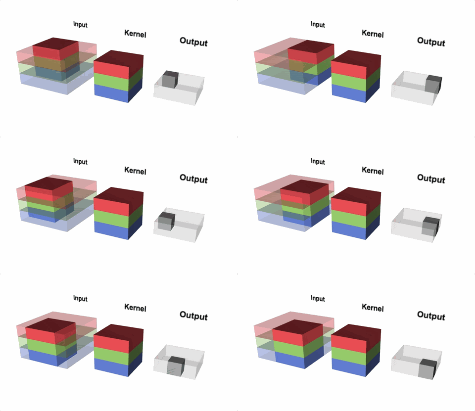
Fully connected layer. After several convolution+pooling blocks have distilled the image into a compact set of feature maps, those maps are flattened and passed through one or more dense layers (Lecture 4's math, unchanged) ending in a classifier — full details in Lecture 14.
4. The Deep CNN Pipeline
Stacking several convolution+pooling blocks before the classifier head gives the standard deep CNN pipeline:
$$\text{Input} \to \text{CL}_1 \to \text{CL}_2 \to \text{CL}_3 \to \text{CL}_4 \to \text{FCL}_1 \to \text{FCL}_2 \to \text{Output}$$where CL = convolutional layer (sparse connectivity — each output unit only "sees" a small local patch of its input) and FCL = fully connected layer (dense connectivity — every output unit sees every input unit).
5. Where Do the Parameters Actually Live?
The two halves of the pipeline behave very differently in terms of parameter count. Convolutional layers hold relatively few parameters — each filter is small (e.g. 3×3 or 5×5) and, crucially, the same filter weights are reused (shared) at every spatial position, so the parameter count doesn't grow with image size. Fully connected layers, by contrast, connect every input unit to every output unit, so their parameter count is the product of two potentially large numbers — and they end up dominating the network's total parameter budget.
Of VGG16's ~140 million total parameters, roughly 85–90% live in the fully-connected layers alone, even though the FC layers are a small fraction of the network's depth (3 of its 19 weight layers). This single fact is what motivated the next generation of architectures — GoogLeNet and ResNet — to shrink or eliminate FC layers entirely (Section 6).
6. Landmark Architectures: Where This Technology Went
Full convolution arithmetic is Lecture 13's job. Here, as a motivating close, is where the 4-layer blueprint led over the following decade of the ImageNet Large Scale Visual Recognition Challenge (ILSVRC).
| Architecture | Year | Depth | Parameters | ImageNet Top-5 error | Signature idea |
|---|---|---|---|---|---|
| AlexNet | 2012 | 5 conv + 3 FC | 62.3 M | 15.4% | ReLU, dropout, heavy data augmentation, split across 2 GPUs |
| VGG16 | 2014 | 16 conv + 3 FC | ~140 M | 7.3% | Uniform 3×3 conv, stride 1 + 2×2 max-pool, stride 2 |
| GoogLeNet | 2015 | Inception modules | 5 M | 6.7% | Multi-scale Inception module, 1×1 convs, no FC layers |
| ResNet-152 | 2015 | 152 layers | ~60 M | 3.57% | Residual/skip connections, F(X)+X |
ImageNet Top-5 error (%)
Parameters (millions)
AlexNet (2012) took a 227×227×3 RGB input through 5 convolutional layers and 3 fully connected layers, split across two GTX 580 GPUs (a hardware constraint of the time), and trained for 5–6 days. It introduced ReLU activations, dropout regularization on the dense layers, and aggressive data augmentation — and its 15.4% Top-5 error was a dramatic improvement over prior hand-engineered feature pipelines. Interestingly, only about 6% of its 62.3 million parameters sit in the convolutional layers, yet those same convolutional layers consume roughly 95% of the network's compute time — parameters and compute are concentrated in opposite ends of the network.
VGG16 (2014) simplified the design space to a single repeated building block — 3×3 convolution, stride 1, followed by 2×2 max-pooling, stride 2 — stacked 16 convolutional layers deep, and it improved Top-5 error to 7.3%. The cost, as Section 5 showed, was a parameter budget of ~140 million, 85% of it sitting in the three FC layers.
GoogLeNet / Inception (2015) attacked that FC parameter cost directly: it uses average pooling instead of flatten+dense at the end, has no fully-connected layers at all, and needs only 5 million parameters — 12× fewer than AlexNet — while still improving accuracy to 6.7% Top-5 error. Its Inception module runs several kernel sizes in parallel within the same layer, capturing features at multiple scales simultaneously. A key trick that keeps this affordable is the 1×1 convolution, used purely to shrink channel depth before an expensive larger convolution:
Input feature map: 56×56×64. Apply five 1×1×64 kernels (each kernel spans the full 64-channel depth but only a single pixel spatially):
$$56\times56\times64 \;\xrightarrow{\;5\ \text{kernels of }1\times1\times64\;}\; 56\times56\times5$$
Spatial resolution (56×56) is untouched — only the channel depth changes, from 64 down to 5, a 64/5 = 12.8× reduction in channel depth before any further, more expensive convolution is applied to the (now much cheaper) 5-channel map.
ResNet (2015), at 152 layers, is described in the course material as the "beginning of the ultra-deep network era." Its defining trick is the residual (skip) connection: \(F(X)+X\) — the input to a small block of conv+ReLU layers is added back to that block's output before the next activation. During backpropagation, the gradient has a direct, unimpeded path through the shortcut, which is exactly what solves the vanishing-gradient-with-depth problem that had made networks this deep untrainable before. The result: 3.57% Top-5 error, below the commonly cited human-level benchmark on this task.
7. Common Pitfalls & Misconceptions
- "Fewer parameters always means a worse model." GoogLeNet (5M params) beats AlexNet (62.3M params) on accuracy — architecture matters more than raw parameter count.
- "More layers always means more parameters." ResNet-152 has roughly 60M parameters despite being far deeper than VGG16 (~140M, only 16 conv layers) — because ResNet has no bulky FC layers and relies on 3×3 convs and global pooling.
- Confusing "sparse connectivity" with "few parameters because the layer is small." A conv layer is sparse because each output unit only connects to a small receptive field, not because the layer has few output units — a conv layer can still produce a huge feature map (e.g. 224×224×64), just with shared weights.
- Forgetting that the input must stay 2D (or 3D with channels). Flattening before the convolutional stack defeats the entire purpose described in Section 1 — flattening only happens once, right before the FC classifier head (Lecture 14).
8. Summary
- A dense network on a 224×224×3 image needs ~150 million weights for just one 1000-unit hidden layer — computationally expensive and overfit-prone.
- MLPs also ignore local spatial structure and have no translation invariance; CNNs fix both with small, shared, spatially-slid filters plus pooling.
- CNN architecture traces directly back to biological vision (Hubel & Wiesel's simple/complex cells) via the Neocognitron, TDNNs, and LeCun's LeNet-5.
- Every CNN is built from the same 4-layer blueprint: Input (kept 2D) → Convolution (filters → ReLU → pooling) → ... → Fully Connected → Output.
- Convolutional layers are parameter-cheap (shared weights); fully-connected layers dominate parameter count — ~85–90% of VGG16's parameters live in its 3 FC layers.
- AlexNet → VGG16 → GoogLeNet → ResNet cut Top-5 ImageNet error from 15.4% to 3.57%, while parameter count moved non-monotonically (62.3M → 140M → 5M → ~60M) — proof that smarter architecture, not raw size, drove the progress.
9. Code: Counting the Parameters
This script reproduces every numeric claim made above — the MLP parameter explosion, the generic conv-layer parameter formula, the 1×1 convolution channel-reduction example, and the landmark-architecture comparison table — as plain, runnable Python (no deep learning framework required).
"""
Lecture 12 -- CNNs: Motivation & Architecture
Reproduces the numeric claims from the lecture: the MLP parameter
explosion on raw images, the conv-layer parameter-count formula, the
1x1 convolution channel-reduction example, and a landmark-architecture
comparison table.
"""

# ---- 1. Why not a dense network on images? ----
H, W, D = 224, 224, 3
flat_inputs = H * W * D
hidden_units = 1000
mlp_weights = flat_inputs * hidden_units

print(f"Flattened 224x224x3 image  -> {flat_inputs:,} inputs")
print(f"Dense layer to {hidden_units} units -> {mlp_weights:,} weights "
      f"(~{mlp_weights/1e6:.1f} million)\n")

# ---- 2. Generic conv-layer parameter count ----
def conv_params(K, D_in, D_k):
    """K x K filter, D_in input channels, D_k output filters (+1 bias each)."""
    return (K * K * D_in * D_k) + D_k

# e.g. 15 filters of 3x3 over a 3-channel input (Lecture 13's example)
p = conv_params(K=3, D_in=3, D_k=15)
print(f"3x3 conv, 3 input channels, 15 filters -> {p:,} parameters "
      f"(compare to the {mlp_weights:,} MLP weights above)\n")

# ---- 3. 1x1 convolution as a channel-depth bottleneck (GoogLeNet trick) ----
in_h, in_w, in_channels = 56, 56, 64
num_1x1_filters = 5
out_shape = (in_h, in_w, num_1x1_filters)
reduction_factor = in_channels / num_1x1_filters
print(f"1x1 conv: {in_h}x{in_w}x{in_channels} -> {out_shape[0]}x{out_shape[1]}x{out_shape[2]}"
      f"  ({reduction_factor:.1f}x channel reduction)\n")

# ---- 4. Landmark architecture comparison ----
architectures = [
    {"name": "AlexNet",   "year": 2012, "params_m": 62.3, "top5_err": 15.4},
    {"name": "VGG16",     "year": 2014, "params_m": 140.0, "top5_err": 7.3},
    {"name": "GoogLeNet", "year": 2015, "params_m": 5.0,  "top5_err": 6.7},
    {"name": "ResNet-152","year": 2015, "params_m": 60.0, "top5_err": 3.57},
]
print(f"{'Model':<12}{'Year':>6}{'Params (M)':>13}{'Top-5 err %':>14}")
for a in architectures:
    print(f"{a['name']:<12}{a['year']:>6}{a['params_m']:>13.1f}{a['top5_err']:>14.2f}")

fewer_params_than_alexnet = architectures[0]["params_m"] / architectures[2]["params_m"]
print(f"\nGoogLeNet uses {fewer_params_than_alexnet:.1f}x fewer parameters than "
      f"AlexNet, yet has lower Top-5 error -- accuracy and parameter count "
      f"are not the same axis.")
⬇ Download lecture-12-cnn-motivation.py More resources for this lecture →