Word Embeddings & Tokenization
To understand language, understand words. To let a machine understand words, turn them into vectors — the whole art is in choosing HOW.
We've now spent four lectures (15–18) building increasingly sophisticated sequence models, and quietly fed them an input \(x_t\) without ever asking, for text, where that vector actually comes from. This lecture fills that gap properly. It's not a detour — the specific weaknesses we'll find in the most obvious answer (Word2Vec's fixed, one-embedding-per-word approach) connect directly to the same bottleneck problem Lecture 18 just raised, and both get solved by the same idea in Lecture 20.
- Explain why words must be converted to numeric vectors before a neural network can process language.
- Build a one-hot encoding by hand and state its two core disadvantages.
- Describe the CBOW and Skip-gram Word2Vec architectures, including the exact matrices involved and what becomes the embedding table after training.
- Explain precisely why Word2Vec produces a static, context-independent embedding — and what problem that causes.
- Describe the out-of-vocabulary problem in word-level tokenization and how sub-word tokenization (BPE, WordPiece) solves it.
- Trace the BPE merge-training algorithm by hand on a small corpus, pair-score round by pair-score round.
1. From Words to Vectors
Every neural network we've studied — feedforward, CNN, RNN, LSTM — computes with numbers: matrix multiplications, dot products, gradients. None of that machinery has any native notion of a "word." So before any language model can do anything, there is one unavoidable question: how do we turn a word into a vector of numbers?
The motivation is exactly this chain of reasoning: to understand language, a model must understand words; the only way a machine can compute with words is if they live in a vector space. This isn't a minor implementation detail — it's foundational. There are more than 7,100 different languages spoken in the world; no fixed rule-based dictionary or hand-coded feature scheme scales to that. What's needed is a general, learnable, numeric representation of "word meaning" that a model can compute with directly. This lecture builds that representation up in three stages: one-hot (naive), Word2Vec (dense, learned), and sub-word tokenization (fixes the vocabulary problem underneath both).
2. One-Hot Encoding
If you already know what a one-hot vector is, skip straight to the worked example below. If not, expand for the definition.
New to this? Expand: what one-hot encoding is
The simplest possible scheme: build a vocabulary of every unique word in your corpus, then represent word \(i\) as a vector of length \(V\) (the vocabulary size) that is 0 everywhere except a single 1 at position \(i\).
Two sentences: "Tokyo is the capital of Japan" and "Mount Fuji is located near Tokyo." Together they contain 10 unique words:
{Tokyo, is, the, capital, of, Japan, Mount, Fuji, Located, near}
So \(\text{Tokyo} = [1,0,0,0,0,0,0,0,0,0]\) and \(\text{is} = [0,1,0,0,0,0,0,0,0,0]\), and so on for every word.
Advantage: trivial to construct — no training required. Disadvantage 1 — no semantic information: the vector encodes nothing about what the word means; it's purely an index. Disadvantage 2 — no notion of similarity: every pair of distinct one-hot vectors is equally far apart (orthogonal). "Tokyo" and "Japan" — closely related — look exactly as dissimilar as "Tokyo" and "banana." There is no way to measure semantic similarity or dissimilarity between words in this representation at all.
3. Word2Vec: Continuous Bag of Words (CBOW)
Word2Vec fixes both one-hot disadvantages at once: it represents words as dense, much lower-dimensional vectors, learned so that semantically similar words end up close together in the embedding space. There are two Word2Vec architectures; CBOW predicts a target word from its surrounding context words.
"[The Wide road shimmered] in the hot sun", window size 2 → target = "wide", context = {The, road, shimmered}
"[The Wide road shimmered in the hot] sun", window size 3 → target = "shimmered", context = {the, wide, road, in, the, hot}
Every one of those (target, context) training pairs is generated by sliding a window across the sentence, one position at a time. Watch it slide below (window size 2, same sentence) — the target word lights up, the words currently inside the window light up as its context, and everything else fades:
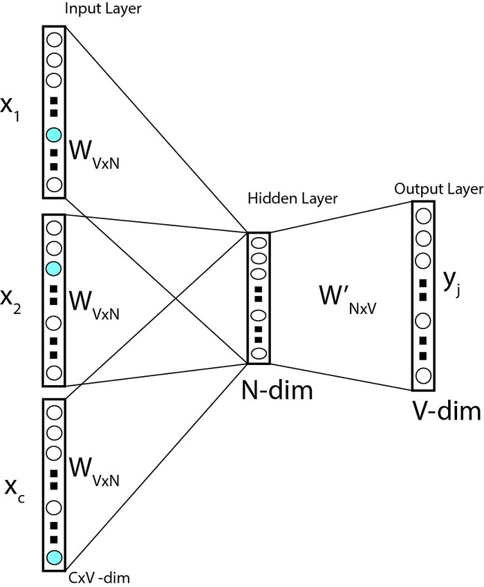
Mechanically: each one-hot context word \(X_i\) (shape \(1\times V\)) is multiplied by a shared weight matrix \(W_{V\times N}\) (\(N\) = embedding dimension, chosen much smaller than \(V\)), and the results for all context words are averaged to produce the hidden layer \(H\) (shape \(1\times N\)):
$$H = \frac{1}{|\text{context}|}\sum_{i} X_i W$$\(H\) is then multiplied by a second matrix \(W'_{N\times V}\) to produce the output layer, and a softmax turns that into a probability distribution over the entire vocabulary for the predicted target word. Training minimizes cross-entropy loss (Lecture 6) between this distribution and the true target word, with weights updated by ordinary backpropagation (Lecture 8) — nothing new algorithmically, just a specific choice of architecture and training task.
After training finishes, \(W_{V\times N}\) — the very matrix used to project one-hot context words into the hidden layer — is the embedding table. Row \(i\) of \(W\) is the learned \(N\)-dimensional embedding for vocabulary word \(i\). The embedding was never designed or hand-specified — it fell out as a byproduct weight matrix of a supervised, next-word-style prediction task. This is the central mechanism behind "how embeddings are generated."
Shrink the vocabulary to just \(V=4\) words — {The, road, shimmered, wide} — with embedding dimension \(N=2\), context {The, road, shimmered}, target "wide". Pick a small illustrative (untrained — this is just to show the mechanics, not a trained model) weight matrix \(W_{4\times2}\), one row per vocabulary word:
$$W=\begin{bmatrix}0.10 & 0.90\\0.80 & 0.20\\0.30 & 0.70\\0.60 & 0.40\end{bmatrix}\begin{matrix}\leftarrow\text{The}\\\leftarrow\text{road}\\\leftarrow\text{shimmered}\\\leftarrow\text{wide}\end{matrix}$$
Since each context word's one-hot vector \(X_i\) has a single 1, the matrix multiply \(X_iW\) (Lecture 4, Section 6's row-by-column rule) just selects that word's row of \(W\) — nothing is summed across rows, because every other row is multiplied by 0:
$$X_{\text{The}}W=[0.10,\,0.90] \qquad X_{\text{road}}W=[0.80,\,0.20] \qquad X_{\text{shimmered}}W=[0.30,\,0.70]$$
Average the three (this is exactly \(H=\frac{1}{|\text{context}|}\sum_i X_iW\) from the equation above), one dimension at a time:
$$H=\left[\frac{0.10+0.80+0.30}{3},\ \frac{0.90+0.20+0.70}{3}\right]=\left[\frac{1.20}{3},\ \frac{1.80}{3}\right]=[\mathbf{0.40},\ \mathbf{0.60}]$$
Now multiply \(H\) (shape \(1\times2\)) by a second weight matrix \(W'_{2\times4}\) (also illustrative) to get one raw score per vocabulary word — again a row-of-\(H\)-dot-column-of-\(W'\) computation:
$$W'=\begin{bmatrix}0.5 & 0.2 & -0.3 & 0.9\\0.1 & 0.4 & \phantom{-}0.6 & -0.2\end{bmatrix}\begin{matrix}\ \\\ \end{matrix}\qquad HW'=[\,0.40(0.5){+}0.60(0.1),\ \ 0.40(0.2){+}0.60(0.4),\ \ 0.40(-0.3){+}0.60(0.6),\ \ 0.40(0.9){+}0.60(-0.2)\,]$$
$$HW'=[\,0.26,\ 0.32,\ 0.24,\ 0.24\,]\quad\text{for}\quad[\text{The},\ \text{road},\ \text{shimmered},\ \text{wide}]$$
Finally, softmax — exponentiate every score, then divide each by the sum of all four exponentials (Lecture 6's normalization):
$$e^{0.26}{\approx}1.2969,\ \ e^{0.32}{\approx}1.3771,\ \ e^{0.24}{\approx}1.2712,\ \ e^{0.24}{\approx}1.2712 \qquad \text{sum}=5.2164$$
$$P(\text{The})=\tfrac{1.2969}{5.2164}{\approx}0.2486\quad P(\text{road})=\tfrac{1.3771}{5.2164}{\approx}0.2640\quad P(\text{shimmered})=\tfrac{1.2712}{5.2164}{\approx}0.2437\quad P(\text{wide})=\tfrac{1.2712}{5.2164}{\approx}0.2437$$
These four numbers sum to 1.0000, as any softmax output must. With these arbitrary starting weights, the model currently favors "road" (0.2640) over the true target "wide" (0.2437) — cross-entropy loss compares this distribution against the one-hot true label \([0,0,0,1]\) and backpropagation (Lecture 8) nudges \(W\) and \(W'\) so that \(P(\text{wide})\) rises on the next pass. Repeated over millions of context windows, this is the entire Word2Vec training loop.
4. Word2Vec: Skip-Gram
Skip-gram runs the same idea in reverse: given the target word, predict each context word individually. For a window size \(w\), this prediction is repeated \(k=2w\) times per target — once per context position.
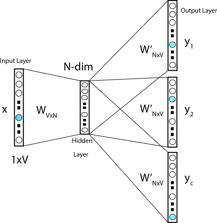
Input is the one-hot target word \(x\) (shape \(1\times V\)); the hidden layer is simply \(H = xW\) (a row lookup into \(W_{V\times N}\), since \(x\) is one-hot); the output is \(H W'\), a length-\(V\) score vector, again turned into a probability distribution via softmax and trained with cross-entropy loss — exactly the same ingredients as CBOW, just with the roles of input and output swapped. As with CBOW, \(W_{V\times N}\) after training is the embedding table.
Reuse the exact same \(W\) and \(W'\) from the CBOW example, but now the target word "wide" is the input, and we want to predict each context word. \(H=xW\) is now just a direct row lookup — no averaging needed, since there's only one input word:
$$H = X_{\text{wide}}W = [\mathbf{0.60},\ \mathbf{0.40}]$$
Multiply by the same \(W'\) to get raw scores over the vocabulary:
$$HW'=[\,0.60(0.5){+}0.40(0.1),\ \ 0.60(0.2){+}0.40(0.4),\ \ 0.60(-0.3){+}0.40(0.6),\ \ 0.60(0.9){+}0.40(-0.2)\,]=[\,0.34,\ 0.28,\ 0.06,\ 0.46\,]$$
Softmax (same procedure as above):
$$e^{0.34}{\approx}1.4050,\ e^{0.28}{\approx}1.3231,\ e^{0.06}{\approx}1.0618,\ e^{0.46}{\approx}1.5842 \qquad \text{sum}=5.3741$$
$$P(\text{The}){\approx}0.2614\quad P(\text{road}){\approx}0.2462\quad P(\text{shimmered}){\approx}0.1976\quad P(\text{wide}){\approx}0.2948$$
This single distribution is compared, in turn, against each of the \(k=3\) true context words — once against the one-hot label for "The", once against "road", once against "shimmered" — producing three separate cross-entropy losses that are summed before backpropagating. That's the sense in which skip-gram makes \(k\) predictions per target: the forward pass runs once, but the loss (and hence the gradient) is accumulated over every context position.
5. The Limitation: Static, Context-Independent Embeddings
Consider: "I went to bank for opening an account" vs. "I went to bank of a river for the walk." The word "bank" means something completely different in each sentence. But Word2Vec assigns the exact same embedding to "bank" in both — because the embedding is just row \(i\) of a fixed table \(W\), looked up by word identity alone, with no way to consult the surrounding sentence.
Word2Vec embeddings are therefore static / context-independent: one word → one fixed vector, no matter what sentence it appears in.
Lecture 20 introduces self-attention, which produces a different embedding for "bank" depending on the words around it — solving exactly this problem by making the representation a function of the whole sentence, not just the word's identity.
6. Tokenization and the Out-of-Vocabulary Problem
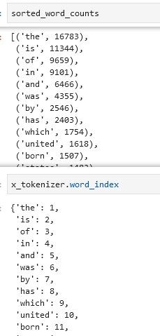
Before any of the above can happen, raw text has to be split into discrete units — tokens — in the first place. The most obvious approach is word-level tokenization: split on spaces and punctuation, count how often each resulting word occurs across the corpus, assign each word an index by frequency rank, and (to keep the vocabulary a manageable size) discard words below some frequency threshold.
Word-level tokenization has a hard failure mode: any word not seen while building the vocabulary — a typo, a rare technical term, a name, a word coined after the vocabulary was frozen — has no index at all. At inference time, the model simply breaks on unseen words; it has nothing to map them to.
7. Sub-Word Tokenization: BPE and WordPiece
Sub-word tokenization fixes the OOV problem by never requiring a word to be a single, indivisible unit in the first place. Instead of building a vocabulary of whole words, it builds a vocabulary of frequently-occurring pieces of words (down to individual characters, in the worst case) — so any string, seen or unseen, can always be represented as some sequence of known pieces.
| Method | Used by | New vocab entries chosen by |
|---|---|---|
| Byte Pair Encoding (BPE) | GPT | highest pair frequency |
| WordPiece | BERT | highest pair score (not raw frequency) |
Both algorithms share the same overall shape: start from individual characters, repeatedly find the best-scoring adjacent pair of symbols currently in use, merge it into a new single vocabulary entry, and repeat — growing the vocabulary one merge at a time until a target size (or no more useful merges) is reached. They differ only in the scoring rule used to pick the winning pair each round.
8. Worked Example: Merge-Training a Sub-Word Vocabulary
Corpus: {huggingface, hugging, face, hug, hugger, learning, learner, learners, learn}. Follow the merge process round by round below (using the ##-continuation convention: ##x marks a character that is not at the start of a word).
Before any merges happen, every word is just its own sequence of characters, with ## marking every character that is not the first one in the word — e.g. "huggingface" → h, ##u, ##g, ##g, ##i, ##n, ##g, ##f, ##a, ##c, ##e.
This gives the starting, purely character-level vocabulary: {##a, ##c, ##e, ##f, ##g, ##i, ##n, ##r, ##s, ##u, f, h, i, l}. Every one of the 9 corpus words is representable right now, just as a long sequence of single-character tokens — sub-word tokenization always starts from a position where nothing is out-of-vocabulary, since individual characters are the fallback.
Look at every pair of adjacent symbols that actually occurs, anywhere in the corpus's current splits, and compute a score for each (BPE scores by raw co-occurrence frequency; WordPiece uses a slightly different formula — the mechanics of "find the best pair, merge it" are identical either way). The full round-1 table:
| Pair | Score |
|---|---|
| h ##u | 0.25 ★ winner |
| ##a ##c | 0.11 |
| ##u ##g | 0.09 |
| ##c ##e | 0.07 |
| ##g ##g | 0.02 |
| f ##a | 0.11 |
| ##g ##i | 0.05 |
| ##g ##e | 0.01 |
| ##i ##n | 0.09 |
| ##e ##r | 0.03 |
| ##n ##g | 0.03 |
| l ##e | 0.07 |
| ##g ##f | 0.09 |
| ##e ##a | 0.06 |
| ##f ##a | 0.11 |
| ##a ##r | 0.06 |
| ##r ##n | 0.05 |
Why "h ##u" wins: scanning down the Score column, 0.25 is the single largest value in the whole table — every other pair tops out at 0.11. That is precisely the merge rule: pick the one pair with the highest score, no matter how many words it appears in or how the rest of the table looks. "h" is immediately followed by "##u" in every word that starts with "hu" — huggingface, hugging, hug, hugger — so this pair racks up occurrences across four of the nine corpus words, driving its score well above any competitor. The algorithm therefore merges h + ##u → a new single vocabulary entry, "hu".
This is the part that actually changes: go back through every word's split and, wherever the symbol "h" is immediately followed by "##u", collapse those two symbols into the single new token "hu". So "huggingface", which started as h, ##u, ##g, ##g, ##i, ##n, ##g, ##f, ##a, ##c, ##e (11 symbols), becomes hu, ##g, ##g, ##i, ##n, ##g, ##f, ##a, ##c, ##e (10 symbols) — one symbol shorter, because two symbols became one. The same replacement happens inside hugging, hug, and hugger. Words that never contained "h ##u" (like face, learning, learner) are untouched by this particular merge. The vocabulary now has one new entry, "hu", alongside all the original single characters — pair scores must be recomputed from scratch on these updated splits, because merging "hu" changes which pairs are even adjacent anymore (e.g. "h ##u" no longer exists as a pair at all — it's been absorbed).
Same procedure as Step 2, just run again on the post-merge splits. Notice "h ##u" has correctly disappeared from the table entirely (it no longer exists as an adjacent pair anywhere), replaced by new pairs like "hu ##g" that only became adjacent because of the round-1 merge:
| Pair | Score |
|---|---|
| hu ##g | 0.09 |
| ##a ##c | 0.11 (tied) |
| ##g ##g | 0.02 |
| f ##a | 0.11 (tied) |
| ##g ##i | 0.05 |
| ##i ##n | 0.09 |
| ##g ##e | 0.01 |
| ##n ##g | 0.03 |
| ##e ##r | 0.03 |
| ##g ##f | 0.09 |
| l ##e | 0.07 |
| ##f ##a | 0.11 (tied) |
| ##e ##a | 0.06 |
| ##r ##n | 0.05 |
| ##a ##r | 0.06 |
Why this round is different: this time there is a three-way tie for the highest score at 0.11 — ##a ##c, f ##a, and ##f ##a are all equally the "best" pair by the scoring rule. Unlike round 1, where one pair was unambiguously ahead, a real implementation needs a tie-breaking convention (e.g. whichever pair was first encountered while scanning the corpus, or alphabetical order — the exact rule differs by library) so that training is reproducible. Whichever of the three wins gets merged into one new vocabulary entry exactly as "hu" was, the corpus is re-split again, and the merge → re-split → re-score cycle repeats for as many rounds as the target vocabulary size requires.
Merge → re-split → re-score, repeated until either no new merges are possible or a target vocabulary size is reached. Each round grows the vocabulary by exactly one new multi-character token — never more — chosen by whichever scoring rule the method uses (pair frequency for BPE, a different pair score for WordPiece). Nothing about the corpus's original words is discarded; every merge is just a compression of two existing adjacent symbols into one new symbol, so the process can always fall back to individual characters for anything it hasn't learned a larger piece for yet — which is exactly what solves the out-of-vocabulary problem from Section 6.
You can replay the same five steps interactively below — useful for testing yourself before moving on:
However far the merge process runs, tokenizing a new string (e.g. "huggingface" itself, or an unseen word) uses greedy longest-match: scan the string and, at each position, take the longest piece that exists in the learned vocabulary, then continue from where that piece ended. Early in training, larger merged pieces like "hu" or "hug" compete with shorter character-level pieces to cover as much of the string as possible in as few tokens as possible — the exact final segmentation depends on precisely which merges have been learned by that point, which is why continuing the merge rounds above (rather than a single fixed split) is the pedagogically important part to understand rigorously.
9. Summary
One-hot (sparse, trivial, but carries no meaning and no notion of similarity) → Word2Vec (dense, low-dimensional, semantically meaningful — but a fixed vector per word, generated as a byproduct weight matrix of CBOW/Skip-gram training) → sub-word tokenization (BPE/WordPiece — solves the out-of-vocabulary problem underneath either representation, by never requiring whole-word units) → Lecture 20 will show how Transformers generate contextual embeddings that change from sentence to sentence, fixing Word2Vec's one remaining weakness: that "bank" always meant the same thing, no matter the sentence.
10. Code: Byte Pair Encoding From Scratch
A toy BPE trainer (word-frequency-based pair counting — the GPT-style algorithm) on the same example corpus, printing each merge as it happens.
"""
Lecture 19 -- Byte Pair Encoding (BPE) merge-training from scratch.
Toy implementation on the same example corpus. Uses classic
BPE (pair FREQUENCY, summed across word counts) -- the algorithm
GPT-style tokenizers use. (WordPiece, used by BERT, scores pairs
differently -- see the lecture notes.)
"""
from collections import defaultdict, Counter

corpus = ["huggingface", "hugging", "face", "hug",
          "hugger", "learning", "learner", "learners", "learn"]
word_freq = Counter(corpus)   # each word appears once here

def split_word(w):
    """Represent a word as a list of symbols; '##' marks a
    non-initial character, following the lecture's convention."""
    return [w[0]] + ["##" + c for c in w[1:]]

splits = {w: split_word(w) for w in word_freq}

def get_vocab(splits):
    v = set()
    for symbols in splits.values():
        v.update(symbols)
    return v

def pair_freqs(splits, word_freq):
    freqs = defaultdict(int)
    for w, symbols in splits.items():
        for a, b in zip(symbols, symbols[1:]):
            freqs[(a, b)] += word_freq[w]
    return freqs

def merge_pair(pair, splits):
    a, b = pair
    merged = a + (b[2:] if b.startswith("##") else b)
    new_splits = {}
    for w, symbols in splits.items():
        out, i = [], 0
        while i < len(symbols):
            if i < len(symbols) - 1 and symbols[i] == a and symbols[i+1] == b:
                out.append(merged); i += 2
            else:
                out.append(symbols[i]); i += 1
        new_splits[w] = out
    return new_splits, merged

print("Initial vocab:", sorted(get_vocab(splits)))

NUM_MERGES = 6
for step in range(1, NUM_MERGES + 1):
    freqs = pair_freqs(splits, word_freq)
    if not freqs:
        break
    best_pair = max(freqs, key=freqs.get)
    splits, merged_token = merge_pair(best_pair, splits)
    print(f"Merge {step}: {best_pair} (freq={freqs[best_pair]}) -> '{merged_token}'")

print("\nFinal splits:")
for w in corpus:
    print(f"  {w:12s} -> {splits[w]}")
⬇ Download lecture-19-bpe.py More resources for this lecture →