Convolution, Padding, Stride & Pooling
The exact arithmetic behind every feature map a CNN ever produces — one sliding dot product, one output-size formula, and the padding, stride and pooling knobs that control it.
Lecture 12 argued convolution is the fix for images, but waved its hands at the actual arithmetic. This lecture makes it precise — exactly how a filter slides, what padding and stride do to the output size, and how pooling shrinks a feature map — because every later CNN lecture (and Lecture 24's convolutional autoencoders) assumes you can compute these sizes without hesitating.
- Define the convolution operation as a sliding elementwise multiply-and-sum, and derive the output-size formula.
- Compute feature-map output sizes by hand for given kernel size, stride and padding, including cases that don't fit.
- Explain why zero padding is used, and why odd-sized kernels are preferred for "same" padding.
- Extend convolution to multi-channel inputs and count the parameters in a convolutional layer.
- Distinguish stride (which reduces resolution) from dilation (which enlarges receptive field without doing so).
- Perform max pooling and Sobel edge detection by hand on small worked examples.
1. The Convolution Operation
A convolutional layer works with a small learnable filter (or kernel) — typically 3×3 or 5×5 — that slides across the input. At every position, the filter and the underlying patch of the input are multiplied elementwise and summed into a single number: a dot product between the flattened filter and the flattened patch. The filter then moves by stride \(S\) pixels and repeats, producing one output value per position — together, these values form the output feature map.
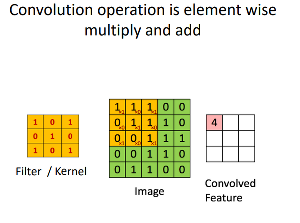
For a square input of size \(W\times W\), a square filter of size \(K\times K\), and stride \(S\):
$$W' = \frac{W-K}{S}+1$$This must come out to a whole number — \((W-K)\) must be exactly divisible by \(S\), otherwise the filter cannot scan the whole image (Section 1.1 below).
Three worked examples, all with input \(H=W=7\):
| Kernel \(K\) | Stride \(S\) | \((W-K)/S\) | Output size |
|---|---|---|---|
| 3 | 1 | 4/1 = 4 | 5×5 |
| 3 | 2 | 4/2 = 2 | 3×3 |
| 3 | 3 | 4/3 = 1.33… | does not fit |
With \(W=7, K=3, S=3\): \(7-3=4\), and \(4/3\) is not an integer. Concretely, the filter's top-left corner can only legally sit at columns 0 and 3 (column 6 would push the filter past the edge of a 7-wide image) — after the window starting at column 3, the next jump of 3 lands at column 6, but a 3-wide filter starting at column 6 needs columns 6,7,8, and column 7 doesn't exist. The last column of the image is never scanned by any window. This is exactly why the formula insists \((W-K)/S\) be a whole number: it's a divisibility check on whether the filter can tile the image exactly.
2. Sliding the Filter: Interactive Walkthrough
To make the sliding mechanism concrete, here is a 3×3 Sobel \(G_x\) filter (introduced formally in Section 7) sliding over a small 5×5 image with a vertical edge — pixels 10 on the left, 80 on the right. With \(W=5, K=3, S=1\), the output-size formula gives \(W'=(5-3)/1+1=3\), so there are exactly 9 valid filter positions.
Every row of the input is \([10,10,10,80,80]\) — a flat block of 10s on the left, a flat block of 80s on the right, and a vertical edge running between columns 2 and 3. At each filter position, multiply the highlighted 3×3 window elementwise by \(G_x=\begin{bmatrix}-1&0&1\\-2&0&2\\-1&0&1\end{bmatrix}\) and add up all nine products.
Position (r=0, c=0) — window = columns 0,1,2, entirely inside the flat left region (every entry is 10):
Row 0: \(10(-1)+10(0)+10(1)=-10+0+10=0\)
Row 1: \(10(-2)+10(0)+10(2)=-20+0+20=0\)
Row 2: \(10(-1)+10(0)+10(1)=-10+0+10=0\)
Output = \(0+0+0=\mathbf{0}\) — no gradient, because the window is perfectly flat.
Position (r=0, c=2) — window = columns 2,3,4, straddling the edge (10, 80, 80 in every row):
Row 0: \(10(-1)+80(0)+80(1)=-10+0+80=70\)
Row 1: \(10(-2)+80(0)+80(2)=-20+0+160=140\)
Row 2: \(10(-1)+80(0)+80(1)=-10+0+80=70\)
Output = \(70+140+70=\mathbf{280}\) — a large response, because the window straddles a sharp intensity change. This is the entire mechanism behind every convolution in this course: slide, multiply elementwise, sum, move on.
You can replay all 9 positions interactively below — useful for testing yourself before moving on:
Input (5×5)
Gx output (3×3)
3. Zero Padding
Every convolution without padding shrinks the feature map (the 7×7 → 5×5 example above). Stack enough layers like that and the feature map vanishes long before the network gets deep. Zero padding adds \(P\) rows/columns of zeros around the border of the input before convolving, which updates the output-size formula:
$$W' = \frac{W-K+2P}{S}+1$$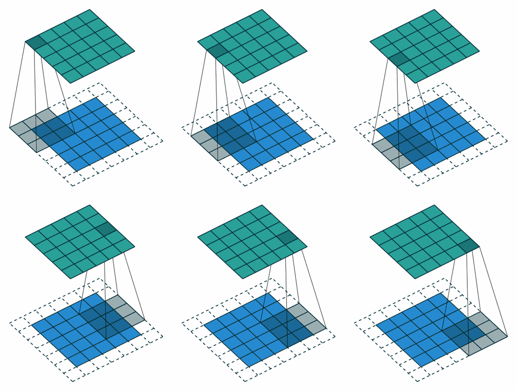
Input \(H=W=7\), \(K=3\), \(S=1\), \(P=1\):
$$W' = \frac{7-3+2(1)}{1}+1 = \frac{6}{1}+1 = 7$$The output stays 7×7 — exactly the input size. This is called "same" padding.
In general, to preserve spatial size exactly with stride 1, you need:
$$P = \frac{K-1}{2}$$The formula \(P=(K-1)/2\) only gives a whole number when \(K\) is odd. Geometrically, an odd-sized filter has a single, well-defined center pixel — the input pixel directly below that center is exactly the pixel the output value "represents," with an equal number of neighboring pixels on every side (left/right, top/bottom). An even-sized filter (e.g. 2×2, 4×4) has no center pixel — its receptive field is asymmetric around any single output position, which complicates padding and interpretation. This geometric symmetry is why 3×3 and 5×5 filters dominate real architectures (recall VGG16's uniform 3×3 choice, Lecture 12).
4. Multi-Channel Convolution
Real images aren't single 2D grids — an RGB image has \(D=3\) channels. A filter for a \(D\)-channel input must itself be \(D\)-channel (e.g. a 3×3×3 filter for an RGB image). The convolution multiplies-and-sums across all channels simultaneously at each spatial position — so, importantly, one filter always produces one 2D output map, regardless of how many input channels it read from.
Depth in the output comes from using multiple filters. Apply \(D_K\) independent filters to the same input, and you get a \(D_K\)-channel output — each filter contributing exactly one of those channels.
Input \(H\times W\times D_I\), \(D_K\) filters of size \(K\times K\):
$$\text{weights} = K\times K\times D_I\times D_K \qquad \text{(} + D_K \text{ biases, one per filter)}$$producing an output feature map of shape \(H'\times W'\times D_K\).
Input \(28\times28\times3\). Apply a single 3×3 filter with 1×1 padding (so, by Section 3's "same" rule, spatial size is preserved):
$$28\times28\times3 \;\xrightarrow{\;1\ \text{filter, }3\times3,\ P{=}1\;}\; 28\times28\times1$$Now apply 15 such filters instead of one:
$$28\times28\times3 \;\xrightarrow{\;15\ \text{filters}\;}\; 28\times28\times15$$The number of filters directly and only controls the output channel depth — spatial size is governed purely by \(K, S, P\) as in Sections 1 and 3.
5. Stride & Dilation
Stride controls how far the filter jumps between positions. Stride 1 (the default) moves the filter one pixel at a time, producing a dense, high-resolution output. Stride 2 moves the filter two pixels at a time — this subsamples the image and roughly halves the output resolution in each dimension, directly reducing the amount of computation in every subsequent layer.
Dilation is a different knob entirely. With dilation factor \(l\), the filter samples every \(l\)-th pixel instead of a contiguous patch — the filter's weights don't change in count, but the pixels they touch spread out. A nominal 3×3 filter with dilation 2 skips every other pixel and so actually spans a 5×5 receptive field, while still only doing 9 multiply-adds.
Standard 3×3, stride 1
Same 3×3 filter, stride 2
Same 3×3 filter, dilation 2 → spans 5×5
Stride shrinks the output resolution as a side effect of subsampling. Dilation enlarges the receptive field without shrinking resolution and without adding parameters — the output size formula from Section 1 is unaffected by dilation on its own. This is the mechanism behind WaveNet-style dilated/causal convolutions, which stack layers of increasing dilation to cover long sequences with very few parameters.
6. Pooling
Pooling spatially down-samples a feature map: fewer values means fewer parameters downstream, less computation, and reduced risk of overfitting. The most common choice is max pooling — typically a 2×2 window with stride 2 — which keeps only the largest value in each window. Pooling uses the same output-size formula as convolution (Section 1), almost always with no padding, and has no learnable parameters at all — it's a fixed, deterministic operation.
Input 4×4:
$$\begin{bmatrix}1&3&2&0\\4&6&1&2\\0&1&3&5\\2&2&2&4\end{bmatrix}$$Stride 2 with a 2×2 window means the four windows are non-overlapping and tile the input exactly — no pixel is read twice. Each output entry is simply the largest of its window's four values:
Top-left window (rows 0–1, cols 0–1) = \(\{1,3,4,6\}\): \(\max(1,3,4,6)=\mathbf{6}\)
Top-right window (rows 0–1, cols 2–3) = \(\{2,0,1,2\}\): \(\max(2,0,1,2)=\mathbf{2}\)
Bottom-left window (rows 2–3, cols 0–1) = \(\{0,1,2,2\}\): \(\max(0,1,2,2)=\mathbf{2}\)
Bottom-right window (rows 2–3, cols 2–3) = \(\{3,5,2,4\}\): \(\max(3,5,2,4)=\mathbf{5}\)
Assembling these four numbers in the same row-major layout as the windows gives the output:
$$\xrightarrow{\;2\times2\ \max,\ S{=}2\;}\; \begin{bmatrix}6&2\\2&5\end{bmatrix}$$
Replay the same four windows interactively below — useful for testing yourself before moving on:
Input (4×4)
Max-pooled output (2×2)
7. Sobel Edge Detection: Convolution in Action
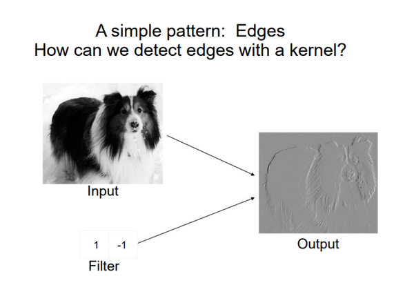
Convolution isn't only for learned CNN filters — the classic, hand-designed Sobel operator is a concrete, motivating example of what a single well-chosen 3×3 filter can compute: image gradients, and from them, edges. Two fixed kernels estimate the gradient in the horizontal (\(x\)) and vertical (\(y\)) directions:
$$G_x=\begin{bmatrix}-1&0&1\\-2&0&2\\-1&0&1\end{bmatrix} \qquad G_y=\begin{bmatrix}-1&-2&-1\\0&0&0\\1&2&1\end{bmatrix}$$Convolving a local neighborhood \(N\) with each kernel gives two numbers, \(S_x = N * G_x\) and \(S_y = N * G_y\), which combine into a gradient magnitude and direction:
$$|\nabla I|=\sqrt{S_x^2+S_y^2} \qquad \theta=\arctan2(S_y, S_x)$$A large \(|\nabla I|\) means pixel intensity is changing sharply at that location — an edge. A small (near-zero) magnitude means the neighborhood is roughly flat.
Neighborhood \(N=\begin{bmatrix}10&10&10\\10&50&80\\10&50&80\end{bmatrix}\) — a region with a bright block in its bottom-right corner.
Multiply every entry of \(N\) by the entry in the matching position of \(G_x\), then add up all nine products, one row at a time:
Row 0: \(10(-1)+10(0)+10(1)=-10+0+10=0\)
Row 1: \(10(-2)+50(0)+80(2)=-20+0+160=140\)
Row 2: \(10(-1)+50(0)+80(1)=-10+0+80=70\)
$$S_x = 0+140+70 = \mathbf{210}$$
Same neighborhood \(N\), now elementwise against \(G_y=\begin{bmatrix}-1&-2&-1\\0&0&0\\1&2&1\end{bmatrix}\):
Row 0: \(10(-1)+10(-2)+10(-1)=-10-20-10=-40\)
Row 1: \(10(0)+50(0)+80(0)=0+0+0=0\)
Row 2: \(10(1)+50(2)+80(1)=10+100+80=190\)
$$S_y = -40+0+190 = \mathbf{150}$$
$$|\nabla I|=\sqrt{S_x^2+S_y^2}=\sqrt{210^2+150^2}=\sqrt{44100+22500}=\sqrt{66600}\approx\mathbf{258.1}$$
(The course slide rounds this to \(\approx258.8\) — a small rounding difference from the source material; either way, this is a large gradient magnitude.) Direction: \(\theta=\arctan2(S_y,S_x)=\arctan2(150,210)\approx35.5°\).
A large \(|\nabla I|\) means pixel intensity is changing sharply at this location → a strong edge is detected at this neighborhood.
Prefer to click through the same computation interactively, one row at a time? Same numbers, same order — useful for testing yourself before moving on:
8. Common Pitfalls
- Forgetting to check divisibility. Always confirm \((W-K+2P)/S\) is a whole number before trusting an output shape — frameworks like Keras/PyTorch will either error out or silently floor/crop, and floor-based cropping quietly discards the last row/column of the input.
- Confusing stride with dilation. Both are integer "spacing" parameters, but stride changes output resolution; dilation changes receptive field size while output resolution (for the convolution itself) stays governed by the same formula.
- Assuming pooling has learnable weights. It doesn't — max pooling is a fixed operation. Only the convolutional filters are trained.
- Forgetting a filter's channel depth must match its input. A filter for a 3-channel input is 3-channel too — a "3×3 filter" over RGB really has 27 weights (3×3×3), not 9.
- Using an even-sized kernel and expecting clean "same" padding. Section 3 showed \(P=(K-1)/2\) only lands on an integer for odd \(K\).
9. Summary
- Convolution is a sliding elementwise multiply-and-sum; output size is \(W'=(W-K)/S+1\), or \(W'=(W-K+2P)/S+1\) with padding — and this must be an integer.
- Zero padding (typically \(P=(K-1)/2\)) preserves spatial size, and only works cleanly for odd-sized filters, which is why 3×3/5×5 kernels dominate.
- A filter always spans the full input channel depth and produces a single 2D output map; stacking \(D_K\) filters produces a \(D_K\)-channel output. Parameter count: \(K\times K\times D_I\times D_K + D_K\).
- Stride subsamples and reduces resolution; dilation enlarges the receptive field for free, without touching parameter count or resolution.
- Max pooling (typically 2×2, stride 2) down-samples with zero learnable parameters, using the same output-size formula as convolution.
- The Sobel operator is hand-designed convolution in action: \(S_x=210, S_y=150, |\nabla I|\approx258.8\) on the worked neighborhood — a strong, unambiguous edge.
10. Code: Convolution Arithmetic, Pooling & Sobel
This NumPy script reproduces every worked number above: the output-size formula and its three K/S test cases, the "same"-padding check, the multi-channel shape/parameter formula, the exact 4×4 max-pooling example, and Sobel \(S_x, S_y\) on the worked neighborhood.
"""
Lecture 13 -- Convolution, Padding, Stride & Pooling
Reproduces: the output-size formula (with/without padding), the
multi-channel conv parameter-count formula, the exact 4x4 max-pooling
worked example, and Sobel Sx/Sy/|grad I| on the worked neighborhood.
"""
import numpy as np

# ---- 1. Output-size formula: W' = (W - K + 2P)/S + 1 ----
def output_size(W, K, S, P=0):
    num = W - K + 2 * P
    if num % S != 0:
        return None  # cannot scan the whole image
    return num // S + 1

for K, S in [(3, 1), (3, 2), (3, 3)]:
    out = output_size(7, K, S)
    print(f"W=7, K={K}, S={S}, P=0 -> {out if out else 'INVALID (does not fit)'}")
print(f"W=7, K=3, S=1, P=1 (same padding) -> {output_size(7, 3, 1, 1)}\n")

# ---- 2. Multi-channel convolution: output shape + parameter count ----
def conv_output(H, W, D_in, K, S, P, D_k):
    Hp, Wp = output_size(H, K, S, P), output_size(W, K, S, P)
    params = (K * K * D_in * D_k) + D_k
    return (Hp, Wp, D_k), params

shape, params = conv_output(28, 28, 3, K=3, S=1, P=1, D_k=15)
print(f"28x28x3 input, 3x3 filter, P=1, 15 filters -> {shape}, {params} params\n")

# ---- 3. Max pooling: exact 4x4 worked example ----
def max_pool(mat, size=2, stride=2):
    mat = np.array(mat)
    out_h = (mat.shape[0] - size)//stride + 1
    out_w = (mat.shape[1] - size)//stride + 1
    out = np.zeros((out_h, out_w))
    for r in range(out_h):
        for c in range(out_w):
            out[r, c] = mat[r*stride:r*stride+size, c*stride:c*stride+size].max()
    return out

X = [[1, 3, 2, 0], [4, 6, 1, 2], [0, 1, 3, 5], [2, 2, 2, 4]]
pooled = max_pool(X)
print("Max pooling 4x4 -> 2x2:\n", pooled)
assert np.array_equal(pooled, [[6, 2], [2, 5]]), "does not match worked example!"

# ---- 4. Sobel edge detection ----
def conv2d_valid(img, kernel):
    img, kernel = np.array(img, float), np.array(kernel, float)
    kh, kw = kernel.shape
    H, W = img.shape
    out = np.zeros((H - kh + 1, W - kw + 1))
    for r in range(out.shape[0]):
        for c in range(out.shape[1]):
            out[r, c] = np.sum(img[r:r+kh, c:c+kw] * kernel)
    return out

Gx = [[-1, 0, 1], [-2, 0, 2], [-1, 0, 1]]
Gy = [[-1, -2, -1], [0, 0, 0], [1, 2, 1]]
N = [[10, 10, 10], [10, 50, 80], [10, 50, 80]]

Sx = conv2d_valid(N, Gx)[0, 0]
Sy = conv2d_valid(N, Gy)[0, 0]
mag = np.sqrt(Sx**2 + Sy**2)
theta = np.degrees(np.arctan2(Sy, Sx))
print(f"\nSobel on N: Sx={Sx:.0f}, Sy={Sy:.0f}, |grad I|={mag:.2f}, theta={theta:.1f} deg")
print("(Course slide rounds |grad I| to ~258.8.)")

# Slide Gx across a 5x5 vertical-edge image (matches the interactive demo)
img5 = [[10, 10, 10, 80, 80]] * 5
print("\nSobel-Gx response over the 5x5 vertical-edge image (3x3 output):\n",
      conv2d_valid(img5, Gx))
⬇ Download lecture-13-convolution-pooling.py More resources for this lecture →